<?xml version="1.0" encoding="utf-8"?><feed xmlns="http://www.w3.org/2005/Atom" ><generator uri="https://jekyllrb.com/" version="3.10.0">Jekyll</generator><link href="https://jboylantoomey.com/feed.xml" rel="self" type="application/atom+xml" /><link href="https://jboylantoomey.com/" rel="alternate" type="text/html" /><updated>2026-03-28T10:40:23+00:00</updated><id>https://jboylantoomey.com/feed.xml</id><title type="html">Justin Boylan-Toomey</title><subtitle>Justin Boylan-Toomey&apos;s personal website.</subtitle><author><name>Justin Boylan-Toomey</name></author><entry><title type="html">Isolated uv Dependency Management in Monorepos</title><link href="https://jboylantoomey.com/post/isolated_uv_dependency_management_in_monorepos" rel="alternate" type="text/html" title="Isolated uv Dependency Management in Monorepos" /><published>2026-01-22T00:00:00+00:00</published><updated>2026-01-22T00:00:00+00:00</updated><id>https://jboylantoomey.com/post/managing-uv-monorepo-envs</id><content type="html" xml:base="https://jboylantoomey.com/post/isolated_uv_dependency_management_in_monorepos"><![CDATA[<p>As a machine learning team we have a number of large projects that have their own repositories, but this is not practical for the large number of smaller, more data science focused projects we carry out. These smaller projects are stored within large thematic monorepos, with each project contained within its own subfolder.</p>

<div class="language-plaintext highlighter-rouge"><div class="highlight"><pre class="highlight"><code>|_monorepo/
  |_project_1/
  |   |_src
  |   |_notebooks
  |   |_models
  |   |_README.md
  |   |_pyproject.toml
  |
  |_ ...
  |
  |_project_n/
  |   |_src
  |   |_notebooks
  |   |_models
  |   |_README.md
  |   |_pyproject.toml
  |
  |_utils/
  |
  |_.gitignore
  |_README.md
  |_pyproject.toml
</code></pre></div></div>
<p>We use the extremely fast <a href="https://docs.astral.sh/uv/">uv</a> package and project manager for our dependency management. Until recently we split more complex monorepos into multiple packages, each dedicated to a specific sub-project, while maintaining common shared dependencies. Sub-project directories are defined as members of a shared <a href="https://docs.astral.sh/uv/concepts/projects/workspaces/">uv workspace</a> in the root level <code class="language-plaintext highlighter-rouge">pyproject.toml</code> file, along with the common shared dependencies of the workspace.</p>

<div class="language-toml highlighter-rouge"><div class="highlight"><pre class="highlight"><code><span class="py">dependencies</span> <span class="p">=</span> <span class="p">[</span>
  <span class="py">"pandas&gt;</span><span class="p">=</span><span class="mf">2.2</span><span class="err">.</span><span class="mi">3</span><span class="s">",</span><span class="err">
</span>  <span class="py">"tqdm&gt;</span><span class="p">=</span><span class="mf">4.67</span><span class="err">.</span><span class="mi">1</span><span class="s">",</span><span class="err">
</span>  <span class="py">"requests&gt;</span><span class="p">=</span><span class="mf">2.32</span><span class="err">.</span><span class="mi">3</span><span class="s">",</span><span class="err">
</span>  <span class="py">"bs4&gt;</span><span class="p">=</span><span class="mf">0.0</span><span class="err">.</span><span class="mi">2</span><span class="s">",</span><span class="err">
</span>  <span class="py">"boto3&gt;</span><span class="p">=</span><span class="mf">1.35</span><span class="err">.</span><span class="mi">68</span><span class="s">",</span><span class="err">
</span>  <span class="py">"lxml&gt;</span><span class="p">=</span><span class="mf">5.3</span><span class="err">.</span><span class="mi">0</span><span class="s">",</span><span class="err">
</span>  <span class="py">"polars&gt;</span><span class="p">=</span><span class="mf">1.30</span><span class="err">.</span><span class="mi">0</span><span class="s">"</span><span class="err">
</span><span class="p">]</span>

<span class="nn">[tool.uv.workspace]</span>
<span class="py">members</span> <span class="p">=</span> <span class="p">[</span>
  <span class="s">"project_1"</span><span class="p">,</span>
  <span class="err">...</span><span class="p">,</span>
  <span class="s">"project_n"</span>
<span class="p">]</span>
</code></pre></div></div>
<p>The default behaviour of running <code class="language-plaintext highlighter-rouge">uv init</code> in a sub-directory, is to add a new <code class="language-plaintext highlighter-rouge">pyproject.toml</code> file to that directory and add the newly created package to the shared uv workspace in the root <code class="language-plaintext highlighter-rouge">pyproject.toml</code>.</p>

<h2 id="the-issue---dependency-conflicts">The Issue - Dependency Conflicts</h2>
<p>However, the uv workspace approach does not scale well with increasing complexity, as sub-projects begin to have conflicting dependency requirements. Especially in cases where code from analytics projects is pushed to git over a period of multiple years and not necessarily maintained.</p>

<p>This is what the uv docs have to say on how to manage complex repositories:</p>

<blockquote>
  <p>Workspaces are intended to facilitate the development of multiple interconnected packages within a single repository. As a codebase grows in complexity, it can be helpful to split it into smaller, composable packages, each with their own dependencies and version constraints.</p>
</blockquote>

<p>And when using a uv workspace may not be the best approach:</p>

<blockquote>
  <p>Workspaces are not suited for cases in which members have conflicting requirements, or desire a separate virtual environment for each member. In this case, path dependencies are often preferable.</p>
</blockquote>

<h2 id="the-solution---isolated-dependencies">The Solution - Isolated Dependencies</h2>

<h3 id="1-remove-the-root-level-uv-definitions-from-repository">1. Remove the root level uv definitions from repository</h3>
<p>If they exist, remove any root level uv related files such as <code class="language-plaintext highlighter-rouge">uv.lock</code> and remove the root level <code class="language-plaintext highlighter-rouge">pyproject.toml</code> file. Each sub-project should still have their own directory, containing a ‘pyproject.toml’ file detailing that projects specific dependencies. The environment for a project can be created by navigating to that project directory using <code class="language-plaintext highlighter-rouge">cd</code> and running <code class="language-plaintext highlighter-rouge">uv sync</code>, this can be better managed using tools like VSCode’s multi-root workspaces as detailed below.</p>

<p>It may also be useful to add the root level uv files to the repositories <code class="language-plaintext highlighter-rouge">.gitignore</code> file, to avoid any accidently created files being pushed to git. The uv specific additions to our <code class="language-plaintext highlighter-rouge">.gitignore</code> file are below, the <code class="language-plaintext highlighter-rouge">/</code> prefix ensures we only ignore root level files:</p>

<div class="language-shell highlighter-rouge"><div class="highlight"><pre class="highlight"><code><span class="c"># monorepo management</span>
/.python-version
/pyproject.toml
/uv.lock
</code></pre></div></div>

<h3 id="2-manage-dependencies-using-multi-root-vscode-workspaces">2. Manage dependencies using multi-root VSCode workspaces</h3>
<p>By default, VSCode only scans the root directory of a project, meaning you have to manually add the interpreter path for each project sub-directory, open each sub-project as an individual VSCode project in it’s own window or update the <code class="language-plaintext highlighter-rouge">$PATH</code> environment variable for VSCode to be able to use each sub-projects isolated <code class="language-plaintext highlighter-rouge">.venv</code> environment.</p>

<p>Multi-root workspaces can streamline working with these isolated environments in VSCode, allowing for multiple isolated projects to be loaded in the same editor window with improved interpreter management.</p>

<p>A multi-root workspace can be configured by adding each sub-project to a <code class="language-plaintext highlighter-rouge">.code-workspace</code> file in the repositories root <code class="language-plaintext highlighter-rouge">.vscode</code> directory. This is a JSON format file which defines the sub-project directories to open as workspace members in a <code class="language-plaintext highlighter-rouge">"folders"</code> list. Each sub-project is represented by a dictionary containing the name of the sub-project and it’s relative directory path. An example definition is below:</p>

<div class="language-json highlighter-rouge"><div class="highlight"><pre class="highlight"><code><span class="p">{</span><span class="w">
	</span><span class="nl">"folders"</span><span class="p">:</span><span class="w"> </span><span class="p">[</span><span class="w">
		</span><span class="p">{</span><span class="w">
			</span><span class="nl">"name"</span><span class="p">:</span><span class="w"> </span><span class="s2">"Project 1"</span><span class="p">,</span><span class="w">
			</span><span class="nl">"path"</span><span class="p">:</span><span class="w"> </span><span class="s2">"../project_1"</span><span class="w">
		</span><span class="p">},</span><span class="w">
                </span><span class="err">...</span><span class="p">,</span><span class="w">
		</span><span class="p">{</span><span class="w">
			</span><span class="nl">"name"</span><span class="p">:</span><span class="w"> </span><span class="s2">"Project n"</span><span class="p">,</span><span class="w">
			</span><span class="nl">"path"</span><span class="p">:</span><span class="w"> </span><span class="s2">"../project_n"</span><span class="p">,</span><span class="w">
		</span><span class="p">}</span><span class="w">
	</span><span class="p">]</span><span class="w">
</span><span class="p">}</span><span class="w">
</span></code></pre></div></div>

<p>To allow VSCode to automatically load the correct environment for each sub-project, a <code class="language-plaintext highlighter-rouge">.vscode/settings.json</code> file is added to the root directory of each sub-project. Each with the below parameters, which inform VSCode that the sub-projects root <code class="language-plaintext highlighter-rouge">.venv</code> environment should be loaded as that sub-projects default Python interpreter.</p>

<div class="language-json highlighter-rouge"><div class="highlight"><pre class="highlight"><code><span class="p">{</span><span class="w">
    </span><span class="nl">"python.defaultInterpreterPath"</span><span class="p">:</span><span class="w"> </span><span class="s2">"${workspaceFolder}/.venv/bin/python"</span><span class="w">
</span><span class="p">}</span><span class="w">
</span></code></pre></div></div>

<p>You can now launch the multi-root workspace in VSCode by navigating to <code class="language-plaintext highlighter-rouge">File &gt; Open workspace from file...</code> and selecting the <code class="language-plaintext highlighter-rouge">.code-workspace</code> file in the repositories root <code class="language-plaintext highlighter-rouge">.vscode</code> directory. This configuration ensures that when you access files within a sub-project, or launch an integrated terminal, the sub projects environment is automatically loaded.</p>]]></content><author><name>Justin Boylan-Toomey</name></author><category term="what I learned today" /><category term="mlops" /><summary type="html"><![CDATA[As a machine learning team we have a number of large projects that have their own repositories, but this is not practical for the large number of smaller, more data science focused projects we carry out. These smaller projects are stored within large thematic monorepos, with each project contained within its own subfolder.]]></summary></entry><entry><title type="html">Relative Citation Ratio (RCR) - How it works and and when to use it.</title><link href="https://jboylantoomey.com/post/relative_citation_ratio_rcr" rel="alternate" type="text/html" title="Relative Citation Ratio (RCR) - How it works and and when to use it." /><published>2026-01-22T00:00:00+00:00</published><updated>2026-01-22T00:00:00+00:00</updated><id>https://jboylantoomey.com/post/rcr</id><content type="html" xml:base="https://jboylantoomey.com/post/relative_citation_ratio_rcr"><![CDATA[<p>The Relative Citation Ratio (RCR) was developed by the National Institute of Health (NIH), to improve the comparability of citation metrics for articles published in different years or across different academic fields. RCR provides a measure of an articles citation rate normalised to compensate for different citation behaviours across academic fields and for time since publication.</p>

<p>Prior to the introduction of the RCR, most field normalised citation metrics used pre-defined ontologies to define research fields. As an example, the Field Citation Ratio (FCR) uses the ANZSRC Field of Research (FoR) ontology in its field normalisation methodology. However, RCR relies on a novel field normalisation approach using an articles co-citation network to dynamically define the field for each article at a more granular local level.</p>

<p>The RCR metric has been found in studies to correlate better with human expert review than raw citation count and metrics using a priori defined field ontologies. Including in our own evaluation benchmarking article metrics with their UK Research Excellence Framework (REF) scores.</p>

<p>In this article we will explore how the RCR is calculated, how to interpret it as a proxy of a publications impact, and some of it’s caveats you should be aware of.</p>

<h2 id="how-is-rcr-calculated">How is RCR Calculated</h2>
<p>The RCR is built using the ratio of two components: The Article Citation Rate (ACR) which is the citation rate of an article of interest normalised by time since publication, and the Expected Citation Rate (ECR) which is the citation rate for articles in a similar field to the article of interest.</p>

\[RCR = \frac{ACR}{ECR}\]

<h3 id="article-citation-rate-acr">Article Citation Rate (ACR)</h3>
<p>The Article Citation Rate (ACR) is calculated as the total citations of the publication of interest (PI), time normalised by dividing by the difference between the most recent year and the PI’s year of publication.</p>

\[ACR = \frac{PI\ Citation\ Count}{Most\ Recent\ Year\ - \ Year\ of\ Publication}\]

<p>This time normalisation of RCR decreases as an article’s citations decline over time, reducing the overall RCR score. Therefore, an articles RCR score should be interpreted as a reflection of its current academic influence and not it’s past influence at time of publication.</p>

<h3 id="expected-citation-rate-ecr">Expected Citation Rate (ECR)</h3>
<p>The Expected Citation Rate (ECR) is calculated using a normalised Field Citation Rate (FCR), which is the expected citations from publications in the same research field as the PI as defined by it’s co-citation network.</p>

<p>A co-citation network consists of all articles cited in articles that also cite the PI. In this case the co-citation network is a proxy for articles in the same field as the research article. The Journal Impact Factor (JIF) is used rather than the citation count of individual articles as this increases the sample size and makes the RCR more stable, with some caveats.</p>

<p>We will get into how the FCR and ECR are calculated but for now it’s probably useful to visualise how the co-citation network is constructed. The below diagram shows the co-citation network for a PI and the journals used to calculate the mean JIF.</p>

<p><img src="https://raw.githubusercontent.com/justinbt1/justinbt1.github.io/refs/heads/main/_posts/media/cocite.png" alt="" /></p>

<p>More concretely the FCR is defined as:
\(Fcr = \frac{\sum{JIF_i}}{N}\)</p>

<ol>
  <li>
    <p>Identify all publications that are cited alongside the PI in citing publications, this gives you the PI’s co-citation network.</p>
  </li>
  <li>
    <p>Sum the Journal Impact Factors (JIFs) of the journal each publication in the co-citation network is published in. If more than one publication is published in the same journal, the journal can be counted multiple times.</p>
  </li>
  <li>
    <p>Finally divide the sum of JIFs by the number of publications in the citation network (N), to get the average JIF.</p>
  </li>
</ol>

<p>The FCR is then normalised to give the ECR used as the denominator in the RCR equation (so many acronyms!). This is done by multiplying the FCR with coefficients from a least squares linear regression model. This model has been trained to predict ACR scores based on the FCR of research publications in the NIH R01 Research Program Grant Program database.</p>

\[ECR^{year} = \hat{B} \times FCR + \hat{a}\]

<h2 id="interpreting-rcr">Interpreting RCR</h2>
<p>The RCR has a global score of 1.0 for average performing articles, with a score higher than one indicating better than average performance when compared to similar articles. The upper limit of the score is boundless, with a minimum score of 0.0.</p>

<p>Like most citation metrics, the distribution for RCR scores is highly skewed following a power law distribution with a long positive tail. This means that the mean of multiple RCR scores can be highly influenced by outlier effects and it may be better to use the median score for some analysis.</p>

<p>The articles in the long positive tail of this distribution can also be analysed to identify articles with exceptional RCR performance. However, care should be taken that the high performance of these articles is not due to score inflation caused any edge case limitations of the metric.</p>

<p>As older papers have more time to accrue citations, the RCR is time normalised by the number of years since publication. However, as citations of a particular work plateau over time, it’s RCR will begin to decrease rapidly with each passing year, even if that paper originally had a high citation rate.</p>

<p>This slow decay of RCR score should be taken into account in any analysis of RCR scores for older publications. With RCR being interpreted as a measure of current, sustained importance rather than the initial impact at time of publication.</p>

<h3 id="co-citation-approach-limitations">Co-citation Approach Limitations</h3>
<p>The RCR approach to field normalisation assumes that articles cited alongside an article of interest are within the same field. This can be confounded when citations or journals are inter-disciplinary, leading to erroneous and misleading RCR scores.</p>

<p>The RCR can also be deflated if an article is frequently cited by articles from fields that typically have a much higher citation rate than the field in which the original article was published. Undesirably penalising an additional citation and an increase in interdisciplinary impact.​ Inversely the RCR can also be inflated, sometimes strongly, if citing articles are frequently from fields with lower citation rates.</p>

<h3 id="guidelines-for-bibliometric-analysis-with-rcr">Guidelines for Bibliometric Analysis with RCR</h3>
<p>General guidelines for use:</p>

<ul>
  <li>
    <p>All citation based bibliometrics have a lag period that allows citations to accrue, I therefore would not recommend using RCR for measuring the performance of portfolio outputs younger than 2 years old.</p>
  </li>
  <li>
    <p>RCR should not be used in isolation to assess organisation or portfolio performance, but as a tool in a wider toolbox.</p>
  </li>
  <li>
    <p>RCR behaviour can be unstable if certain edge cases are present, these effects are smoothed out if aggregated robustly over a large number of data points.</p>
  </li>
  <li>
    <p>As citation based bibliometrics follow a power-law or log-normal distribution, RCR can be sensitive to outlier effects, consequently median instead of arithmetic mean may need to be used when aggregating at a portfolio level.​</p>
  </li>
  <li>
    <p>Citation driven bibliometrics such as RCR are subject to the effects of several confounding variables, such as journal ranking, document type and gender. This should be considered during interpretation and normalised if necessary.​</p>
  </li>
  <li>
    <p>Care should be taken when comparing RCR across research organisations or funders, it may be necessary to normalise on several factors including amount funded, proportion of impact and size of research institutions.</p>
  </li>
  <li>
    <p>Any caveats and context should be communicated alongside any bibliometric evaluation.</p>
  </li>
</ul>]]></content><author><name>Justin Boylan-Toomey</name></author><category term="bibliometrics" /><category term="statistics" /><summary type="html"><![CDATA[The Relative Citation Ratio (RCR) was developed by the National Institute of Health (NIH), to improve the comparability of citation metrics for articles published in different years or across different academic fields. RCR provides a measure of an articles citation rate normalised to compensate for different citation behaviours across academic fields and for time since publication.]]></summary></entry><entry><title type="html">Migrating Sub-Directory While Preserving Git History</title><link href="https://jboylantoomey.com/post/migrating-subfolder-while-preserving-git-history" rel="alternate" type="text/html" title="Migrating Sub-Directory While Preserving Git History" /><published>2026-01-19T00:00:00+00:00</published><updated>2026-01-19T00:00:00+00:00</updated><id>https://jboylantoomey.com/post/git-migration</id><content type="html" xml:base="https://jboylantoomey.com/post/migrating-subfolder-while-preserving-git-history"><![CDATA[<p>Recently we decided to open source some code we use internally for bibliometrics analysis, and share it in a public repository. However this code existed as a sub-folder in our analytics monorepo, so the question was how could we migrate the contents of that sub-folder to a new repo while preserving the git history for only those files?</p>

<p>It turns out this can be easily done using the <code class="language-plaintext highlighter-rouge">git-filter-repo</code> library, I’ve shared the steps below for anyone who needs to do the same.</p>

<h3 id="prepare-the-repositories">Prepare the Repositories</h3>
<p>First create a completely empty repo on GitHub and clone it locally, then make a fresh clone of the repo containing the sub-folder of code to be migrated.</p>

<h3 id="filter-repository-contents-and-git-history">Filter Repository Contents and Git History</h3>
<p>To use the <code class="language-plaintext highlighter-rouge">git-filter-repo</code> library with Python, first you will need to install it into an active Python environment using pip or pipx:</p>
<div class="language-shell highlighter-rouge"><div class="highlight"><pre class="highlight"><code>pip <span class="nb">install </span>git-filter-repo
</code></pre></div></div>
<p>Then you can run the below command in the freshly cloned original repository to filter out all content from the repo and the git history, preserving only the history and files you wish to migrate:</p>
<div class="language-shell highlighter-rouge"><div class="highlight"><pre class="highlight"><code>git filter-repo <span class="nt">--path</span> path_to_subdirectory/
</code></pre></div></div>
<p>You may then want to tidy up the repository a bit, moving the sub-directory files to the top level of the repository, update or add a README, etc.</p>

<h3 id="migrate-to-new-repository">Migrate to New Repository</h3>
<p>The <code class="language-plaintext highlighter-rouge">filter-repo</code> command should have also removed the repositories origin from git, you can check this by running:</p>
<div class="language-shell highlighter-rouge"><div class="highlight"><pre class="highlight"><code>git remote <span class="nt">-v</span>
</code></pre></div></div>
<p>Once satisfied that the origin is no longer pointing at the original repository you can update it to point to the new empty one:</p>
<div class="language-shell highlighter-rouge"><div class="highlight"><pre class="highlight"><code>git remote add origin https://github.com/your_org/new_repo.git
</code></pre></div></div>
<p>You can then push the code to the new repostory:</p>
<div class="language-shell highlighter-rouge"><div class="highlight"><pre class="highlight"><code>git push origin main
</code></pre></div></div>

<p><em>Hope this was helpful, or at least interesting!</em></p>]]></content><author><name>Justin Boylan-Toomey</name></author><category term="what I learned today" /><category term="mlops" /><summary type="html"><![CDATA[Recently we decided to open source some code we use internally for bibliometrics analysis, and share it in a public repository. However this code existed as a sub-folder in our analytics monorepo, so the question was how could we migrate the contents of that sub-folder to a new repo while preserving the git history for only those files?]]></summary></entry><entry><title type="html">Merging Git Repos into an Existing Repository on GitHub</title><link href="https://jboylantoomey.com/post/merging-git-repos-into-an-existing-repository-on-github" rel="alternate" type="text/html" title="Merging Git Repos into an Existing Repository on GitHub" /><published>2025-11-28T00:00:00+00:00</published><updated>2025-11-28T00:00:00+00:00</updated><id>https://jboylantoomey.com/post/merging-git-repos%20copy</id><content type="html" xml:base="https://jboylantoomey.com/post/merging-git-repos-into-an-existing-repository-on-github"><![CDATA[<p>Recently we’ve launched a new project seeking to improve data quality of our impact reporting. This project has grown out of a number of smaller projects, some of which have their own git repository on GitHub. For project and code management reasons we have decided to combine these into a single monorepo, bringing all components of this project into a single place.</p>

<p>The challenge was that we wanted to:</p>

<ul>
  <li>Merge multiple repositories into one that already existing repository.</li>
  <li>Preserve the Git history of the repositories we merge.</li>
  <li>Avoid merge conflicts with pre-existing monorepo code.</li>
  <li>Migrate open and closed issues to the new repository as we use GitHub Projects to manage our work.</li>
  <li>Avoid tightly coupling dependancies between projects.</li>
</ul>

<p>In this article we go through how we merged each of these smaller project repositories into the main monorepo, including solves for the challenges we encountered.</p>

<h2 id="monorepo-structure">Monorepo Structure</h2>
<p>The monorepo for our project is broken into directories each containing separate self contained sub-projects.</p>

<div class="language-plaintext highlighter-rouge"><div class="highlight"><pre class="highlight"><code>|_monorepo/
  |_project_component_1/
  |   |_src
  |   |_notebooks
  |   |_models
  |   |_README.md
  |   |_pyproject.toml
  |
  |_ ...
  |
  |_project_component_n/
  |   |_src
  |   |_notebooks
  |   |_models
  |   |_README.md
  |   |_pyproject.toml
  |
  |_utils/
  |
  |_.gitignore
  |_README.md
  |_pyproject.toml
</code></pre></div></div>

<p>Each projects is loosely coupled, with code that is mostly independent of the others, with some core shared utility code.</p>

<h2 id="prepare-for-merge">Prepare for Merge</h2>
<p>Before merging we needed to also prepare each of the project repositories to avoid issues with the merge. As an example the simplified general structure of one of our project repositories is:</p>

<div class="language-plaintext highlighter-rouge"><div class="highlight"><pre class="highlight"><code>|_project_repo/
  |_models/
  |_pipeline/
  |_notebooks/
  |_.gitignore
  |_README.md
  |_pyproject.toml
</code></pre></div></div>

<p>However if we attempt to merge this with our monorepo there will be multiple merge conflicts. To avoid this we moved everything for transfer to inside a new parent directory with the project name.</p>

<div class="language-plaintext highlighter-rouge"><div class="highlight"><pre class="highlight"><code>|_project_repo/
  |_project_name/
    |_models/
    |_pipeline/
    |_notebooks/
    |_README.md
    |_pyproject.toml
</code></pre></div></div>

<p>We also dropped the <code class="language-plaintext highlighter-rouge">.gitignore</code> as this already existed at the top level of the monorepo we hoped to merge into. This can all be achieved using the below commands within a <strong>new branch</strong> in the local copy of the project repository.</p>

<div class="language-sh highlighter-rouge"><div class="highlight"><pre class="highlight"><code>git branch <span class="nt">-b</span> prep_for_move
<span class="nb">rm</span> <span class="nt">-f</span> .gitignore
<span class="nb">mkdir </span>project_name
git <span class="nb">mv</span> <span class="nt">-k</span> <span class="k">*</span> .<span class="k">*</span> project_name
git add <span class="k">*</span>
git commit <span class="nt">-m</span> <span class="s2">"Prepare for move"</span>
git push <span class="nt">--set-upstream</span> origin prep_for_move
</code></pre></div></div>

<p>We used <code class="language-plaintext highlighter-rouge">git mv</code> to avoid moving the <code class="language-plaintext highlighter-rouge">.git</code> directory from the top level of the local project repository. The flag <code class="language-plaintext highlighter-rouge">-k</code> avoids raising an error caused by trying to move the <code class="language-plaintext highlighter-rouge">project_name</code> directory to within itself.</p>

<h2 id="merge-the-repositories">Merge the Repositories</h2>
<p>Now for the part where we actually merged each individual project repo into the existing monorepo.</p>

<p>This was done by running the below commands from within the local git directory for the monorepo. First make sure that the local is set to the main branch of the monorepo, usually this is called main.</p>

<div class="language-sh highlighter-rouge"><div class="highlight"><pre class="highlight"><code>git checkout origin main
</code></pre></div></div>

<p>Then we needed to add the project repo as a remote on the local monorepo git repository. Make sure you replace <code class="language-plaintext highlighter-rouge">project_repo</code> with the name of the repo you wish to merge and <code class="language-plaintext highlighter-rouge">owner</code> with your GitHub account or org name.</p>

<div class="language-sh highlighter-rouge"><div class="highlight"><pre class="highlight"><code>git remote add <span class="nt">-f</span> project_repo https://github.com/owner/project_repo
</code></pre></div></div>

<p>Then merge the <code class="language-plaintext highlighter-rouge">prep_for_move</code> branch into the <code class="language-plaintext highlighter-rouge">main</code> monorepo branch. The <code class="language-plaintext highlighter-rouge">--allow-unrelated-histories</code> flag allows the merging of histories despite the repos having no common ancestor.</p>

<div class="language-sh highlighter-rouge"><div class="highlight"><pre class="highlight"><code>git merge <span class="nt">-m</span> <span class="s2">"Merging project_repo"</span> project_repo/prep_for_move <span class="nt">--allow-unrelated-histories</span>
</code></pre></div></div>

<p>We then removed the project repo as a remote repository to avoid any later complications.</p>

<div class="language-sh highlighter-rouge"><div class="highlight"><pre class="highlight"><code>git remote <span class="nb">rm </span>project_repo
</code></pre></div></div>

<p>Then finally we pushed the merged changes and histories to the main branch of the monorepo.</p>

<div class="language-sh highlighter-rouge"><div class="highlight"><pre class="highlight"><code>git push
</code></pre></div></div>

<p>Note: If there is a lot of code, which is likely given we are merging an entire repo, the push may time out. This can often be resolved by increasing the POST buffer size in the Git configuration.</p>

<div class="language-sh highlighter-rouge"><div class="highlight"><pre class="highlight"><code>git config http.postBuffer 524288000
</code></pre></div></div>

<h2 id="bulk-migrate-github-issues">Bulk Migrate GitHub Issues</h2>
<p>To bulk migrate GitHub issues from the project repo to the new monorepo, we used the <code class="language-plaintext highlighter-rouge">gh</code> GitHub CLI tool. See <a href="https://cli.github.com/">here</a> for install instructions, you can then authenticate using <code class="language-plaintext highlighter-rouge">gh auth login</code> to connect to your GitHub account.</p>

<p>Then if you are in the local git directory for the project repo you can move (add to target repo, remove from project repo) the issues using the below command.</p>

<p>Though you will need to change <code class="language-plaintext highlighter-rouge">owner/monorepo</code> to match your target repo.</p>

<div class="language-sh highlighter-rouge"><div class="highlight"><pre class="highlight"><code>gh issue list <span class="nt">--json</span> number <span class="nt">--state</span> <span class="s2">"all"</span> | jq <span class="nt">-c</span> <span class="s1">'.[].number'</span> | <span class="k">while </span><span class="nb">read </span>issue<span class="p">;</span> <span class="k">do
    </span><span class="nb">echo</span> <span class="s2">"Trying to transfer issue number: </span><span class="nv">$issue</span><span class="s2">"</span>
    gh issue transfer <span class="nv">$issue</span> owner/monorepo
    <span class="nb">echo</span> <span class="s2">"Transfer successful"</span>
<span class="k">done</span>
</code></pre></div></div>

<p>What’s happening here:</p>

<ul>
  <li>In the first section, the gh issue list — json number command retrieves a list of all issue numbers on repo_old as a JSON array. The option –state “all” means both open and closed issues are listed, to migrate only the active issues use –state “open”.</li>
  <li>The next section uses the jq lightweight JSON processor to extract the number value and flatten the JSON into a flat bash array.</li>
  <li>Then this array is iterated over in a while loop, which uses the gh issue transfer command to transfer each issue based on it’s issue number to the target repo.</li>
</ul>

<h2 id="tidying-things-up">Tidying Things Up</h2>
<p>Finally we tidied up the project repository by deleting the temporary <code class="language-plaintext highlighter-rouge">prep_for_move</code> branch and then archived the repository.</p>

<p><em>Hope this was helpful, or at least interesting!</em></p>]]></content><author><name>Justin Boylan-Toomey</name></author><category term="what I learned today" /><category term="mlops" /><summary type="html"><![CDATA[Recently we’ve launched a new project seeking to improve data quality of our impact reporting. This project has grown out of a number of smaller projects, some of which have their own git repository on GitHub. For project and code management reasons we have decided to combine these into a single monorepo, bringing all components of this project into a single place.]]></summary></entry><entry><title type="html">Is The Average of Averages The Same as The Overall Average?</title><link href="https://jboylantoomey.com/post/is-the-average-of-averages-the-same-as-the-overall-average" rel="alternate" type="text/html" title="Is The Average of Averages The Same as The Overall Average?" /><published>2025-06-13T00:00:00+00:00</published><updated>2025-06-13T00:00:00+00:00</updated><id>https://jboylantoomey.com/post/mean-of-means</id><content type="html" xml:base="https://jboylantoomey.com/post/is-the-average-of-averages-the-same-as-the-overall-average"><![CDATA[<p>There is a simple question that always seems to crop up when discussing everything from analytics dashboards to parallel computation. That is, when you have multiple groups of data (e.g., from different sources or processes), each with its own average, can you simply average those individual averages to get the true average across all the data?</p>

<p>The short answer to this question is no, the longer answer is it depends. The average of multiple averages over sets of elements is only guaranteed to be the same as the average of all elements when:</p>

<ul>
  <li>The cardinality (number of elements) of each averaged set are the same.</li>
  <li>The trivial and rare case where all set averages equal to zero.</li>
</ul>

<p>Let’s have a look at why, the mean of the values in the below set is 5.5:</p>

\[a = \{ 1, 2, 3, 4, 5, 6, 7, 8, 9, 10 \}\]

<p>However, if we break this set into three arbitrary sets (a, b, c) and take the mean of each we get a combined average across all sets of 5.17:</p>

\[a = \{1, 2, 3\}\]

\[b = \{4, 5, 6\}\]

\[c = \{7, 8, 9, 10\}\]

\[(\bar{a} + \bar{b} + \bar{c}) / 3 = 5.17\]

<p>The discrepancy is due to the combined average not accounting for the number of elements in each set. This discrepancy will become larger as the difference between the set sizes increases.</p>

<p>We can instead use weighted averages to reliably calculate the overall average of all elements across all set. The weighted averages of sets (a, b, c) can be calculated using the below process:</p>

<ul>
  <li>For each set calculate a weight, this can be found by dividing the number of elements in a set by the total number of elements in all of the sets combined.</li>
  <li>Weight the average of each set by finding the product between the sets average value and the associated weight.</li>
  <li>Sum each of the weighted averages to give a combined average that represents the true average value of all elements in all sets.</li>
</ul>

<p>We can apply the above process to our sets (a, b, c) to calculate the weighted averages, which when summed give the true overall average of 5.5.</p>

\[\bar{a}\ (3 / 10) = 0.6\]

\[\bar{b}\ (3 / 10) = 1.5\]

\[\bar{c}\ (4 / 10) = 3.4\]

\[0.6 + 1.5 + 3.4 = 5.5\]]]></content><author><name>Justin Boylan-Toomey</name></author><category term="data science" /><category term="statistics" /><summary type="html"><![CDATA[There is a simple question that always seems to crop up when discussing everything from analytics dashboards to parallel computation. That is, when you have multiple groups of data (e.g., from different sources or processes), each with its own average, can you simply average those individual averages to get the true average across all the data?]]></summary></entry><entry><title type="html">Postgres Not Equal Only Returns Non-Null Values</title><link href="https://jboylantoomey.com/post/postgres-not-equal-only-returns-non-null-values" rel="alternate" type="text/html" title="Postgres Not Equal Only Returns Non-Null Values" /><published>2025-06-06T00:00:00+00:00</published><updated>2025-06-06T00:00:00+00:00</updated><id>https://jboylantoomey.com/post/postgres-not-equal</id><content type="html" xml:base="https://jboylantoomey.com/post/postgres-not-equal-only-returns-non-null-values"><![CDATA[<p>As part of an analysis I recently ran a PostgreSQL query to return results filtered to remove rows in which the status column contained values not equal to “started”. However after running the below query using the &lt;&gt; operator I noticed it returned far less rows than expected.</p>

<div class="language-sql highlighter-rouge"><div class="highlight"><pre class="highlight"><code><span class="k">SELECT</span> <span class="n">publication_id</span><span class="p">,</span> <span class="n">start_date</span><span class="p">,</span> <span class="n">department</span><span class="p">,</span> <span class="n">pub_status</span>
<span class="k">FROM</span> <span class="n">pub_schema</span><span class="p">.</span><span class="n">publications</span>
<span class="k">WHERE</span> <span class="n">pub_status</span> <span class="o">&lt;&gt;</span> <span class="s1">'Started'</span><span class="p">;</span>
</code></pre></div></div>

<p>When I investigated this was due to the pub_status column containing mostly Nulls, which were not being returned in the query results. With only rows containing a non-Null status value other than ‘Started’ being returned.</p>

<p>As mentioned in the Postgres <a href="https://www.postgresql.org/docs/current/functions-comparison.html">functions comparison documentation</a> this is due to the not equal to operator (&lt;&gt; or !=) treating Nulls as non-comparable and thereby ignoring and excluding them from the query. This is a common pitfall across most databases as following the SQL Standard if any value on either side of an operator is a Null the equation should evaluate to false, including Null = Null.</p>

<p>This is actually quite logical with the value of Null being by definition unknown, this makes an equivalence with a null value unknowable, as explained in this quote from the <a href="https://en.wikipedia.org/wiki/Null_(SQL)">Wikipedia page</a> on Nulls in SQL:</p>

<p><strong>A null should not be confused with a value of 0. A null indicates a lack of a value, which is not the same as a zero value. For example, consider the question “How many books does Adam own?” The answer may be “zero” (we know that he owns none) or “null” (we do not know how many he owns).</strong></p>

<p>To include rows in the result where status can also be Null, I ended up using the IS DISTINCT FROM predicate (below). This predicate treats Nulls as comparable values rather than unknowns. Meaning it will return Nulls alongside with any other rows that do not equal ‘Started’ (or any other specified criteria).</p>

<div class="language-sql highlighter-rouge"><div class="highlight"><pre class="highlight"><code><span class="k">SELECT</span> <span class="n">publication_id</span><span class="p">,</span> <span class="n">start_date</span><span class="p">,</span> <span class="n">department</span><span class="p">,</span> <span class="n">pub_status</span>
<span class="k">FROM</span> <span class="n">pub_schema</span><span class="p">.</span><span class="n">publications</span>
<span class="k">WHERE</span> <span class="n">pub_status</span> <span class="k">IS</span> <span class="k">DISTINCT</span> <span class="k">FROM</span> <span class="s1">'Started'</span><span class="p">;</span>
</code></pre></div></div>]]></content><author><name>Justin Boylan-Toomey</name></author><category term="databases" /><summary type="html"><![CDATA[As part of an analysis I recently ran a PostgreSQL query to return results filtered to remove rows in which the status column contained values not equal to “started”. However after running the below query using the &lt;&gt; operator I noticed it returned far less rows than expected.]]></summary></entry><entry><title type="html">Neo4j Super Node Performance Issues</title><link href="https://jboylantoomey.com/post/neo4j-super-node-performance-issues" rel="alternate" type="text/html" title="Neo4j Super Node Performance Issues" /><published>2024-02-26T00:00:00+00:00</published><updated>2024-02-26T00:00:00+00:00</updated><id>https://jboylantoomey.com/post/super-nodes</id><content type="html" xml:base="https://jboylantoomey.com/post/neo4j-super-node-performance-issues"><![CDATA[<p>We recently developed a multi-billion relationship scale knowledge graph, representing the wider academic landscape. How we developed the data pipeline to build this graph in Neo4j is a story in itself, one I may write up here or on the <a href="https://medium.com/wellcome-data">Wellcome Data blog</a>. This post however focuses on a specific database modelling issue that has caused us severe query performance issues, the issue of low cardinality “super nodes”.</p>

<h2 id="what-are-super-nodes">What are Super Nodes?</h2>
<p>Nodes with a large number of relationships (there is no formal number, but roughly 100k or more relationships) are known as “super nodes”. These high degree nodes may occur either due to the underlying structure of the real world network the graph represents, or the presence of low cardinality node types (nodes with a small number of possible categorical values) in the data model. The possible underlying causes of super nodes are well explained by David Allen in his blog post <a href="https://medium.com/neo4j/graph-modeling-all-about-super-nodes-d6ad7e11015b">here</a>.</p>

<p>For us it was a case of our data outgrowing our original data model, with performance issues surfacing only once we had fully populated our knowledge graph. These issues presented as very slow queries when traversing or filtering relationships on certain node types, sometimes taking several days for relatively simple queries to run. On investigation I noticed these node types contained many nodes that were acting as super nodes in our graph.</p>

<p>Super nodes can impact performance in a number of ways:</p>

<ul>
  <li>
    <p>The default token lookup index Neo4j creates for each relationship only contains relationship type information. This means Neo4j has to assess all connections from a node it is traversing in a query, so it can identify the next node in the traversal.</p>
  </li>
  <li>
    <p>Dense nodes can also increase the number of relationships within a given relationship type, which may make queries slower.</p>
  </li>
  <li>
    <p>When creating a new relationship between nodes in the database, it is common practices to use MERGE to check such a relationship does not already exist. Neo4j will check if the relationship yet exists, which will be slower where there are a large number of relationships.</p>
  </li>
  <li>
    <p>Super nodes can also lead to issues with scalability, as everything in the network is close to everything else, making the data hard to break into partitions.</p>
  </li>
</ul>

<h2 id="field-of-research-example">Field of Research Example</h2>
<p>As an example our data model included Field of Research (FoR) nodes, which each represent a broad category of scientific research as defined by ANZSRC. There are 100 million Publication nodes in our database, each linked to one or more of the 176 Field of Research nodes.</p>

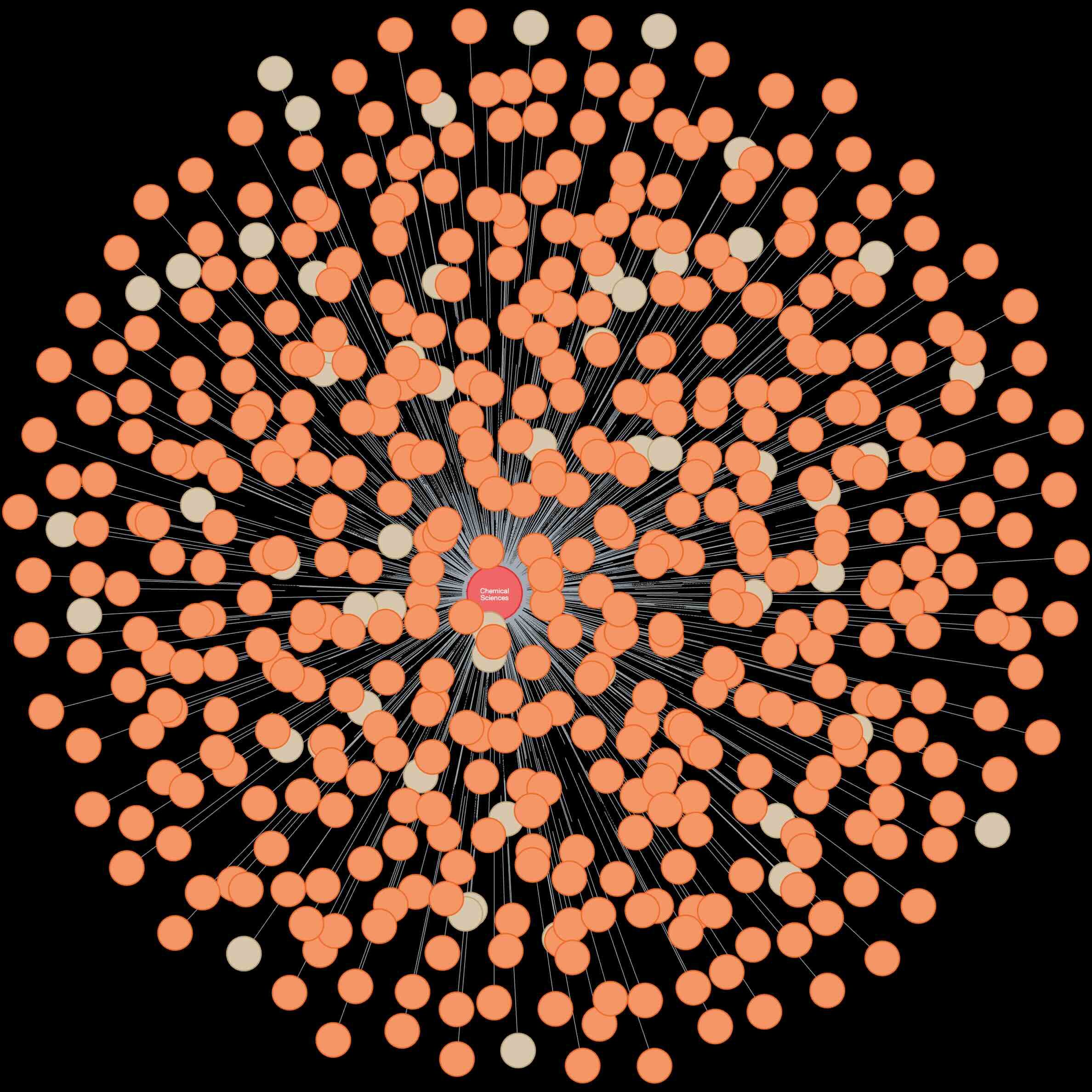
<p align="center">
  <img src="https://raw.githubusercontent.com/justinbt1/justinbt1.github.io/refs/heads/main/images/blog/snode.jpeg" />
  <br />A Field of Research super node, with a sample of it's connected nodes displayed.
</p>

<p>In a best case scenario, where the number of relationships is evenly distributed, each field of research would be linked to approximately 568,000 publications. However in reality publications from a small number of fields of research are over represented in our database, meaning millions of publications may have a relationship with a single field of research.</p>

<p>For example the below Cypher query returns all researchers who have published clinical science papers in 2020:</p>

<div class="language-cypher highlighter-rouge"><div class="highlight"><pre class="highlight"><code><span class="k">MATCH</span><span class="w">
</span><span class="ss">(</span><span class="py">r:</span><span class="n">Researcher</span><span class="ss">)</span><span class="o">-</span><span class="ss">[</span><span class="py">a:</span><span class="n">AUTHORED</span><span class="ss">]</span><span class="o">-&gt;</span><span class="ss">(</span><span class="py">p:</span><span class="n">Publication</span> <span class="ss">{</span><span class="nl">year</span><span class="dl">:</span><span class="m">2020</span><span class="ss">})</span>
<span class="o">-</span><span class="ss">[]</span><span class="o">-</span><span class="ss">(</span><span class="py">f:</span><span class="n">FieldOfResearch</span> <span class="ss">{</span><span class="py">name:</span><span class="s2">"Clinical Sciences"</span><span class="ss">})</span>
<span class="k">RETURN</span> <span class="n">r</span>
</code></pre></div></div>

<p>This query would take an extremely long time to execute as several million unindexed relationships between publications and the clinical science FoR node need to be checked during query execution.</p>

<h2 id="improving-perfomance">Improving Perfomance</h2>
<h3 id="query-refactoring">Query Refactoring</h3>
<p>The simplest way we can improve performance is to refactor our queries to make them more efficient. One of the simplest ways to do this is to ensure both the relationship type and directionality are defined in the Cypher query.</p>

<div class="language-cypher highlighter-rouge"><div class="highlight"><pre class="highlight"><code><span class="c1">//Non-directional and undefined</span>
<span class="k">MATCH</span><span class="ss">(</span><span class="py">p:</span><span class="n">Publication</span><span class="ss">)</span><span class="o">-</span><span class="ss">[]</span><span class="o">-</span><span class="ss">(</span><span class="py">p:</span><span class="n">FieldOfResearch</span><span class="ss">)</span>

<span class="c1">//Directional and defined</span>
<span class="k">MATCH</span><span class="ss">(</span><span class="py">p:</span><span class="n">Publication</span><span class="ss">)</span><span class="o">-</span><span class="ss">[</span><span class="py">l:</span><span class="n">LINKED</span><span class="ss">]</span><span class="o">-&gt;</span><span class="ss">(</span><span class="py">p:</span><span class="n">FieldOfResearch</span><span class="ss">)</span>
</code></pre></div></div>

<p>Unfortunately this does not help in our use case as all of the super nodes in our model have mono-directional, single type relationships with their related nodes.</p>

<h3 id="indexing-relationships">Indexing Relationships</h3>
<p>Neo4j does index relationships by default using a token lookup index that only contains type information for each index rather than information on which nodes they connect. However since version 4.3, Neo4j also supports indexing on relationship properties, this can be used to reduce the number of relationships that have to be checked during query execution.</p>

<p>For example the relationship between a Field of Research and a Publication node might have a publication_year property,  which could be used as a filter to reduce the number of relationships required in a query by filtering to a specific year:</p>

<div class="language-cypher highlighter-rouge"><div class="highlight"><pre class="highlight"><code><span class="k">MATCH</span><span class="ss">(</span><span class="py">p:</span><span class="n">Publication</span><span class="ss">)</span><span class="o">-</span><span class="ss">[</span><span class="py">l:</span><span class="n">LINKED</span> <span class="ss">{</span><span class="nl">year</span><span class="dl">:</span><span class="m">2020</span><span class="ss">}]</span><span class="o">-&gt;</span><span class="ss">(</span><span class="py">p:</span><span class="n">FieldOfResearch</span><span class="ss">)</span>
</code></pre></div></div>

<p>This moderately improves performance of some queries where the use of this property is an appropriate filter. However in our data model there are no properties that could reasonably be used as filters, and these relationships are often queried in bulk reducing any performance advantage.</p>

<h3 id="refactoring-super-nodes-to-node-properties">Refactoring Super Nodes to Node Properties</h3>
<p>Another option, that swaps our unreasonable execution time for a more reasonable increase in spatial complexity, is to refactor the super nodes in our data model to properties on their related nodes. This is especially appealing given the super nodes in our model are categorical, with single type, unidirectional relationships.</p>

<p>For example a relationship between a publication and a field of research super node, could be set instead as a property on the Publication node. These properties could then be indexed to further improve query performance, and the redundant super nodes and their many relationships could then (carefully) be removed from the graph.</p>

<p>Refactoring super nodes to properties did improve the performance of our queries, particularly those that include, but do not filter on the new super node property. There was a wrinkle though, the incoming relationships on the super nodes were one to many relationships, meaning the new super node properties have multiple values.</p>

<p>For example a publication node could be linked to multiple field of research nodes:</p>

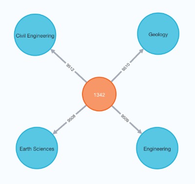
<p align="center">
  <img src="https://raw.githubusercontent.com/justinbt1/justinbt1.github.io/refs/heads/main/images/blog/pub_node.jpg" />
  <br />A Publication node linked to multiple Field of Research super nodes.
</p>

<p>The properties of these field of research nodes now need to be set as properties on the publication node. Initially we used a list property to store these values, with a single list property for each of these values. This however is still not optimal as Neo4j does not currently support indexing on the elements within lists, making these slow to query at scale.</p>

<h3 id="full-text-indexes-to-the-rescue">Full Text Indexes to The Rescue</h3>
<p>Neo4j does however support full text indexes for string properties and make them fully searchable using the Apache Lucene search and indexing library. Neo4j also allows the specification of the analyzer Lucene should use to tokenise the text for index and querying. One of the available analyzers is “whitespace” which breaks text into individual searchable word tokens based on the Java whitespace standard.</p>

<p>By converting our list elements to a single string type property, we were able to leverage the full text index to drastically improve query times when filtering by any of the list elements. To convert the lists to a string, we first replaced the white space in each element with an _ then merged the elements into a single long space separated lower case string.</p>

<p>For example the field of research list property:</p>

<div class="language-python highlighter-rouge"><div class="highlight"><pre class="highlight"><code><span class="n">field_of_research</span><span class="p">:[</span>
  <span class="s">"Civil Engineering"</span><span class="p">,</span>
  <span class="s">"Geology"</span><span class="p">,</span>
  <span class="s">"Earth Sciences"</span><span class="p">,</span>
  <span class="s">"Engineering"</span>
<span class="p">]</span>
</code></pre></div></div>
<p>Was converted to the string property:</p>
<div class="language-python highlighter-rouge"><div class="highlight"><pre class="highlight"><code><span class="n">field_of_research</span><span class="p">:</span><span class="s">"civil_engineering geology earth_sciences engineering"</span>
</code></pre></div></div>
<p>These new string properties were then indexed with the full text index configured to use the whitespace analyzer, using the below Cypher procedure:</p>
<div class="language-cypher highlighter-rouge"><div class="highlight"><pre class="highlight"><code><span class="k">CREATE</span> <span class="n">FULLTEXT</span> <span class="k">INDEX</span> <span class="n">field_of_research_fultext</span>
<span class="n">FOR</span><span class="w"> </span><span class="ss">(</span><span class="py">p:</span><span class="n">Publication</span><span class="ss">)</span>
<span class="k">ON</span> <span class="n">EACH</span> <span class="ss">[</span><span class="n">p.field_of_research</span><span class="ss">]</span>
<span class="n">OPTIONS</span> <span class="ss">{</span>
  <span class="py">indexConfig:</span> <span class="ss">{</span>
    <span class="sb">`fulltext.analyzer`</span><span class="err">:</span> <span class="s1">'whitespace'</span>
  <span class="ss">}</span>
<span class="ss">}</span>
</code></pre></div></div>
<p>Making it possible to use full text search to efficiently filter by the element in each string property.</p>

<div class="language-cypher highlighter-rouge"><div class="highlight"><pre class="highlight"><code><span class="k">CALL</span> <span class="n">db.index.fulltext.queryNodes</span><span class="ss">(</span>
  <span class="s2">"field_of_research_fultext"</span><span class="ss">,</span>
  <span class="s2">"earth_sciences"</span>
<span class="ss">)</span>
<span class="k">YIELD</span> <span class="n">node</span>
<span class="k">MATCH</span><span class="w"> </span><span class="ss">(</span><span class="n">node</span><span class="ss">)</span><span class="o">&lt;-</span><span class="ss">[]</span><span class="o">-</span><span class="ss">(</span><span class="py">r:</span><span class="n">Researcher</span><span class="ss">)</span>
<span class="k">RETURN</span> <span class="n">node</span><span class="ss">,</span> <span class="n">r</span>
</code></pre></div></div>
<h3 id="performance-improvement">Performance Improvement</h3>
<p>Migrating field of research from it’s own Field of Research node type to a full-text indexed property on each publication node has drastically improved query times. With queries seeking to find all publication nodes in a given year, linked to specific fields of research have gone from taking nearly a day to execute to a few seconds.</p>]]></content><author><name>Justin Boylan-Toomey</name></author><category term="databases" /><category term="network analysis" /><summary type="html"><![CDATA[We recently developed a multi-billion relationship scale knowledge graph, representing the wider academic landscape. How we developed the data pipeline to build this graph in Neo4j is a story in itself, one I may write up here or on the Wellcome Data blog. This post however focuses on a specific database modelling issue that has caused us severe query performance issues, the issue of low cardinality “super nodes”.]]></summary></entry><entry><title type="html">Multimodal Document Classification</title><link href="https://jboylantoomey.com/post/multimodal-document-classification" rel="alternate" type="text/html" title="Multimodal Document Classification" /><published>2020-10-10T00:00:00+00:00</published><updated>2020-10-10T00:00:00+00:00</updated><id>https://jboylantoomey.com/post/multimodal_docs</id><content type="html" xml:base="https://jboylantoomey.com/post/multimodal-document-classification"><![CDATA[<p>The automatic classification of documents remains an important and only partially solved information management problem within the upstream oil and gas industry. Companies in this sector have typically amassed vast repositories of unstructured data measuring in the range of tens to thousands of terabytes. <a href="https://www.cgg.com/sites/default/files/2020-11/cggv_0000029162.pdf">An estimated 80% of all data within the upstream oil and gas industry is stored within large unstructured document repositories</a>.</p>

<p>Retrieving relevant documents from these large unstructured data repositories is a major challenge for the industry, with some reports suggesting that <a href="https://www.sciencedirect.com/science/article/pii/S2405656118301421">geoscientists and engineers spend over 50% of their time searching for data</a>. Locating specific data such as porosity and permeability logs, well trajectories and composite wireline logs can be challenging.</p>

<p>Many of the document types found in such repositories are vital to informing exploration and risk management decisions, as well as to ensuring regulatory compliance. If crucial data is omitted from exploration models due to difficulties in its retrieval, this can lead to costly dry exploration wells or jeopardise the safety of a company’s operations.</p>

<h2 id="document-classification">Document Classification</h2>
<p>Automated document classification algorithms aid information retrieval from these repositories by automatically identifying document types. These classifiers act in a similar manner to static search queries, which when combined with key word search, allow results to be refined to only include the data types a user is seeking to retrieve. The predicted classifications when used more broadly can also assist in providing data management oversight of the data within these repositories.</p>

<p>Recently, supervised machine learning has been widely used to create these algorithmic classifiers. With the machine learning algorithm learning a document classification prediction function from a pre-labelled corpus of representative documents. Historically these classifiers can learn document classifications at a granular level based on a documents text content or at a higher level based on image representations of their pages.</p>

<h2 id="multi-modal-approach">Multi-Modal Approach</h2>
<p>The majority of documents in the upstream oil and gas domain are multimodal, meaning they rely on multiple channels to communicate information to the reader, <a href="https://dl.acm.org/doi/10.1109/TPAMI.2018.2798607">relying on both textual and visual modalities for communication</a>. For example most documents contain free text, often alongside text stored in tables, captions and figures. This text gives documents their semantic meaning and in many cases conveys the majority of the information.</p>

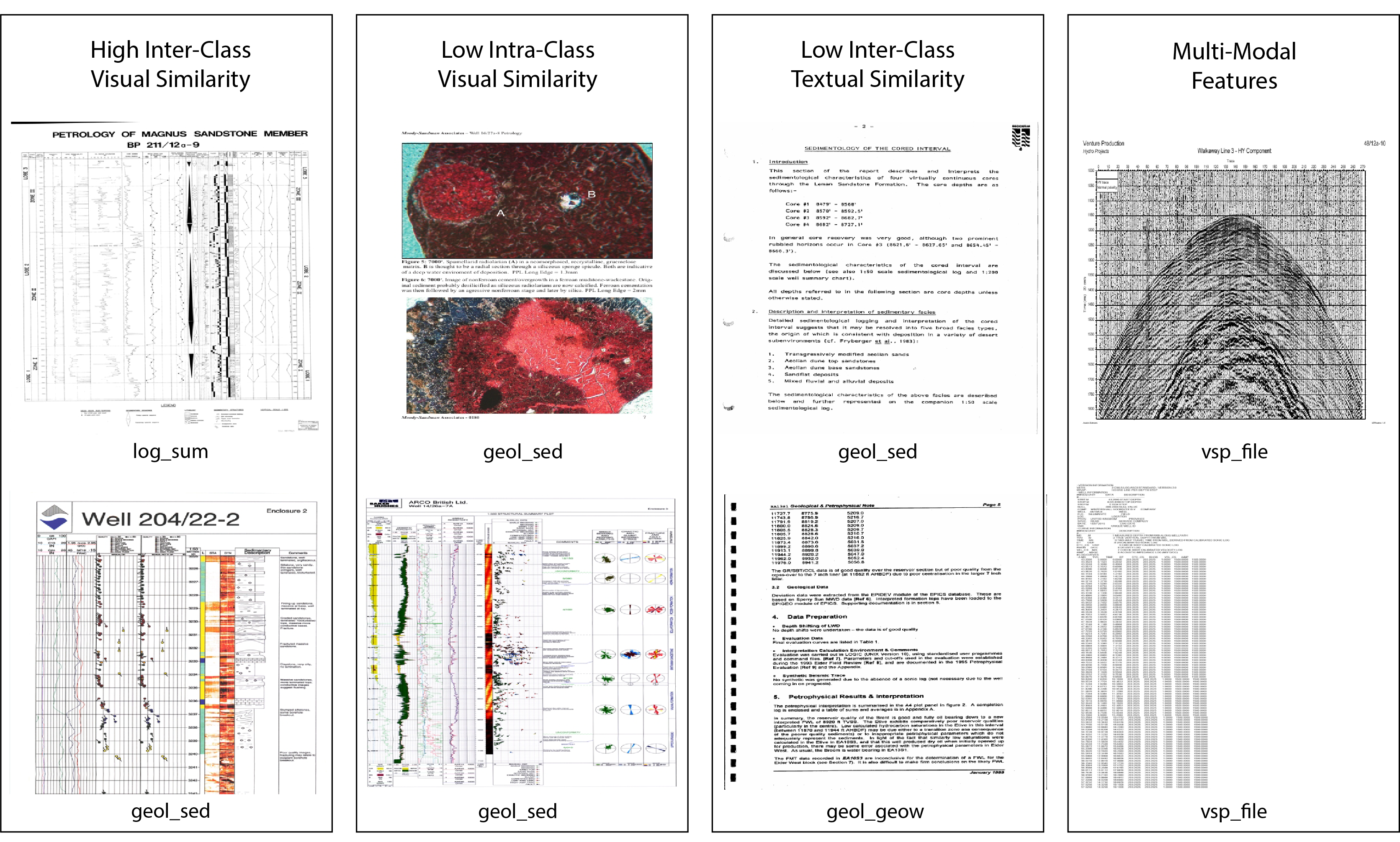
<p>However visual features such as a documents layout, colour distribution, text formatting, charts and image content provide supplementary meaning alongside text based features. In some cases visual features will convey the majority of the information, examples of exploration documents that primarily communicate information visually include sample images, maps, technical diagrams, seismic sections and wireline logs.</p>

<p align="center">
  <img src="https://raw.githubusercontent.com/justinbt1/Multimodal-Document-Classification/refs/heads/main/report/media/page_samples.png" />
  <br />Figure 1: Sample NDR Page Images
</p>

<p>Contemporary uni-modal document classification models used in the industry often rely on features from a single modality, either textual or visual. However, it is difficult to build a robust high performance uni-modal classifier over such a complex multi-modal dataset. For example, document classifiers making use of visual features extracted from page images may underperform due to the high inter-class similarity or intra-class variance of some document page images.</p>

<p>Document classifiers that rely on features from only the text modality tend to outperform image based classifiers at classifying oil and gas documents at a granular level. However these classifiers only perform well when enough text data is present in a document, some documents in the corpus such as diagrams and sample images do not contain any text making them impossible to classify using a text based approach alone. Other documents contain text that may be repeated across multiple document types. For example an oil well name and location being the only text data within visually different images such as between a map and a technical schematic, making them semantically similar but visually distinct.</p>

<p>This blog post explores using a multi-modal approach to oil and gas document classification, combining both text and visual modalities to create a more robust classifier for oil and gas exploration and production documents. With the hypothesis that a multi-modal classification approach combining text and visual feature input streams, will outperform a classifier trained on features from a single modality such as text or visual features.</p>

<h2 id="data-pre-processing">Data Pre-processing</h2>
<p>The document corpus for this project comes from the UK National Data Repository (NDR), an online repository maintained by the UK Oil and Gas Authority for the storage of petroleum related information and samples. The NDR contains hundreds of thousands of documents, representing 65 document types defined by labels known as CS8 Codes.</p>

<p>For the purposes of our experiment a document corpus was created by taking a random sample of approximately 1000 documents from each of 6 key document classes present in the NDR, with each document’s provided CS8 Code being used as a classification label. The document classes selected for inclusion in this dataset were; geological end of well reports (geol_geow), geological sedimentary reports (geol_sed), general geophysical reports (gphys_gen), well log summaries (log_sum), pre-site reports (pre_site) and vertical seismic profile files (vsp_file).</p>

<h3 id="feature-extraction">Feature Extraction</h3>
<p>As this is a new dataset, the text and page image features needed to be extracted from each document in the NDR corpus, for use as training, validation and test data for evaluating each of the classification models. The raw documents were downloaded manually via the free to access NDR website where they are available under an open data license and processed using a feature extraction pipeline.</p>

<p>Unfortunately features were not successfully extracted from all documents, some older Microsoft Office documents could not be processed, while others were corrupt or had non-standard file formats. Several documents also did not contain any text content and therefore lack a text feature set.</p>

<table>
  <thead>
    <tr>
      <th>Document Class</th>
      <th>Extracted Image Features</th>
      <th>Extracted Text Features</th>
      <th>Either Features</th>
    </tr>
  </thead>
  <tbody>
    <tr>
      <td>geol_geow</td>
      <td>1609</td>
      <td>1477</td>
      <td>1609</td>
    </tr>
    <tr>
      <td>geol_sed</td>
      <td>1013</td>
      <td>964</td>
      <td>1013</td>
    </tr>
    <tr>
      <td>gphys_gen</td>
      <td>1041</td>
      <td>876</td>
      <td>1041</td>
    </tr>
    <tr>
      <td>log_sum</td>
      <td>1051</td>
      <td>887</td>
      <td>1051</td>
    </tr>
    <tr>
      <td>pre_site</td>
      <td>1154</td>
      <td>1053</td>
      <td>1154</td>
    </tr>
    <tr>
      <td>vsp_file</td>
      <td>673</td>
      <td>621</td>
      <td>673</td>
    </tr>
    <tr>
      <td><strong>Total:</strong></td>
      <td>6541</td>
      <td>5878</td>
      <td>6541</td>
    </tr>
  </tbody>
</table>

<p align="center">
  <br />Count of Feature Sets Extracted per Document.
</p>

<h3 id="text-pre-processing">Text Pre-Processing</h3>
<p>The text feature dataset consists of a vector of integers T for each document representing the first 2,000 informative terms following text extraction and pre-processing. To create each vector, each document’s text first had to be extracted. Text extraction from ascii format files was achieved using native Python. For Microsoft Office files and PDF files with an embedded searchable text layer text was extracted using Apache Tika Server. For scanned PDF files without an embedded text layer and image format files, text was extracted using the Tesseract OCR Engine.</p>

<div class="language-python highlighter-rouge"><div class="highlight"><pre class="highlight"><code><span class="k">def</span> <span class="nf">start_tika_server</span><span class="p">(</span><span class="n">tika_path</span><span class="p">):</span>
    <span class="n">command</span> <span class="o">=</span> <span class="sa">f</span><span class="s">'java -cp "</span><span class="si">{</span><span class="n">tika_path</span><span class="si">}</span><span class="s">" org.apache.tika.server.TikaServerCli '</span> \
    <span class="s">'--port 80 --host 127.0.0.1'</span>
    <span class="n">tika_server</span> <span class="o">=</span> <span class="n">subprocess</span><span class="p">.</span><span class="n">Popen</span><span class="p">(</span>
        <span class="n">command</span><span class="p">,</span> <span class="n">stdout</span><span class="o">=</span><span class="n">subprocess</span><span class="p">.</span><span class="n">DEVNULL</span><span class="p">,</span> <span class="n">stderr</span><span class="o">=</span><span class="n">subprocess</span><span class="p">.</span><span class="n">DEVNULL</span>
    <span class="p">)</span>

    <span class="k">try</span><span class="p">:</span>
        <span class="n">requests</span><span class="p">.</span><span class="n">get</span><span class="p">(</span><span class="s">'http://127.0.0.1:80/tika'</span><span class="p">)</span>
    <span class="k">except</span> <span class="n">requests</span><span class="p">.</span><span class="n">exceptions</span><span class="p">.</span><span class="nb">ConnectionError</span> <span class="k">as</span> <span class="n">e</span><span class="p">:</span>
        <span class="k">raise</span> <span class="nb">SystemExit</span><span class="p">(</span><span class="sa">f</span><span class="s">'Unable to connect to Tika Server. </span><span class="si">{</span><span class="n">e</span><span class="si">}</span><span class="s">'</span><span class="p">)</span>

    <span class="k">return</span> <span class="n">tika_server</span>
  
<span class="k">def</span> <span class="nf">extract_text</span><span class="p">(</span><span class="nb">file</span><span class="p">):</span>
    <span class="n">tika_response</span> <span class="o">=</span> <span class="n">requests</span><span class="p">.</span><span class="n">put</span><span class="p">(</span>
        <span class="n">url</span><span class="o">=</span><span class="sa">f</span><span class="s">'http://127.0.0.1:80/tika'</span><span class="p">,</span>
        <span class="n">data</span><span class="o">=</span><span class="nb">file</span><span class="p">,</span>
        <span class="n">headers</span><span class="o">=</span><span class="p">{</span>
            <span class="s">'X-Tika-PDFOcrStrategy'</span><span class="p">:</span> <span class="s">'no_ocr'</span><span class="p">,</span>
            <span class="s">'X-Tika-OCRLanguage'</span><span class="p">:</span> <span class="s">'eng'</span><span class="p">,</span>
            <span class="s">'X-Tika-OCRTimeout'</span><span class="p">:</span> <span class="s">'1500'</span><span class="p">,</span>
            <span class="s">'Accept'</span><span class="p">:</span> <span class="s">'text/plain'</span>
        <span class="p">},</span>
        <span class="n">timeout</span><span class="o">=</span><span class="mi">1500</span>
    <span class="p">)</span>

    <span class="n">tika_response</span> <span class="o">=</span> <span class="p">{</span>
        <span class="s">'content'</span><span class="p">:</span> <span class="n">tika_response</span><span class="p">.</span><span class="n">text</span><span class="p">,</span>
        <span class="s">'status'</span><span class="p">:</span> <span class="n">tika_response</span><span class="p">.</span><span class="n">status_code</span>
    <span class="p">}</span>

    <span class="k">return</span> <span class="n">tika_response</span>
</code></pre></div></div>

<p>The raw text extracted from each document was case folded to lower case and tokenized using the pre-trained Word Punkt tokenizer available in the NLTK library, into a sequence of individual tokens. Any tokens with low semantic value were then dropped from the sequence, including non-word tokens such as numbers and punctuation, as well as frequently occurring stopwords. Each token was then lemmatized to it’s base form using the Word Net lemmatizer in NLTK, this reduces dimensionality while preserving the semantic meaning of each token term.</p>

<div class="language-python highlighter-rouge"><div class="highlight"><pre class="highlight"><code><span class="k">def</span> <span class="nf">text_processing</span><span class="p">(</span><span class="n">text</span><span class="p">):</span>
    <span class="n">lemmatizer</span> <span class="o">=</span> <span class="n">nltk</span><span class="p">.</span><span class="n">stem</span><span class="p">.</span><span class="n">WordNetLemmatizer</span><span class="p">()</span>
    <span class="n">text</span> <span class="o">=</span> <span class="n">text</span><span class="p">.</span><span class="n">casefold</span><span class="p">()</span>
    <span class="n">text</span> <span class="o">=</span> <span class="n">text</span><span class="p">.</span><span class="n">translate</span><span class="p">(</span><span class="n">text</span><span class="p">.</span><span class="n">maketrans</span><span class="p">({</span><span class="s">'</span><span class="se">\'</span><span class="s">'</span><span class="p">:</span> <span class="bp">None</span><span class="p">,</span> <span class="s">'-'</span><span class="p">:</span> <span class="s">' '</span><span class="p">}))</span>
    <span class="n">text</span> <span class="o">=</span> <span class="n">nltk</span><span class="p">.</span><span class="n">word_tokenize</span><span class="p">(</span><span class="n">text</span><span class="p">)</span>
    <span class="n">clean_tokens</span> <span class="o">=</span> <span class="p">[]</span>

    <span class="k">for</span> <span class="n">token</span> <span class="ow">in</span> <span class="n">text</span><span class="p">:</span>
        <span class="k">if</span> <span class="n">token</span> <span class="ow">in</span> <span class="n">nltk</span><span class="p">.</span><span class="n">corpus</span><span class="p">.</span><span class="n">stopwords</span><span class="p">.</span><span class="n">words</span><span class="p">(</span><span class="s">'english'</span><span class="p">):</span>
            <span class="k">continue</span>
        <span class="k">if</span> <span class="ow">not</span> <span class="n">token</span><span class="p">.</span><span class="n">isalpha</span><span class="p">():</span>
            <span class="k">continue</span>
        <span class="k">if</span> <span class="nb">len</span><span class="p">(</span><span class="n">token</span><span class="p">)</span> <span class="o">&lt;</span> <span class="mi">2</span><span class="p">:</span>
            <span class="k">continue</span>

        <span class="n">token</span> <span class="o">=</span> <span class="n">lemmatizer</span><span class="p">.</span><span class="n">lemmatize</span><span class="p">(</span><span class="n">token</span><span class="p">)</span>
        <span class="n">clean_tokens</span><span class="p">.</span><span class="n">append</span><span class="p">(</span><span class="n">token</span><span class="p">)</span>

    <span class="n">clean_string</span> <span class="o">=</span> <span class="s">' '</span><span class="p">.</span><span class="n">join</span><span class="p">(</span><span class="n">clean_tokens</span><span class="p">)</span>

    <span class="k">return</span> <span class="n">clean_string</span>
</code></pre></div></div>

<p>The processed tokens were then converted to integers, this was achieved by creating a vocabulary set V containing all unique tokens extracted from each document and mapping each to a unique integer value v. The first 2,000 processed tokens for each document are then mapped to their corresponding v integer value in V to create a vector of integers T for each document. Any vectors with less than 2,000 integers are padded with 0 so that |T| = 2,000 giving a consistent input size for our models.</p>

<h3 id="image-pre-processing">Image Pre-Processing</h3>
<p>The visual feature dataset consists of sequences of JPEG images, with each sequence S containing image representations of the first ten pages of each document in the corpus. For documents in a non-image file format the pages were converted to image representations.</p>

<p>For PDF format documents each page was converted to a single JPEG image using the Poppler PDF rendering library.</p>

<div class="language-python highlighter-rouge"><div class="highlight"><pre class="highlight"><code><span class="kn">from</span> <span class="nn">pdf2image</span> <span class="kn">import</span> <span class="n">convert_from_bytes</span>

<span class="k">with</span> <span class="nb">open</span><span class="p">(</span><span class="n">file_properties</span><span class="p">.</span><span class="n">file_path</span><span class="p">,</span> <span class="s">'rb'</span><span class="p">)</span> <span class="k">as</span> <span class="n">pdf_file</span><span class="p">:</span>
  <span class="n">pdf_bytes</span> <span class="o">=</span> <span class="n">pdf_file</span><span class="p">.</span><span class="n">read</span><span class="p">()</span>
 
<span class="n">page_images</span> <span class="o">=</span> <span class="n">convert_from_bytes</span><span class="p">(</span><span class="n">pdf_bytes</span><span class="p">,</span> <span class="n">dpi</span><span class="o">=</span><span class="mi">300</span><span class="p">,</span> <span class="n">size</span><span class="o">=</span><span class="p">(</span><span class="mi">500</span><span class="p">,</span> <span class="mi">500</span><span class="p">))</span>
</code></pre></div></div>

<p>For raw text format files a new blank image with all white pixels was created using a standard A4 page size of 1748 x 2480 pixels and the documents text content was fitted to and overlayed on each blank page image. For documents with less than ten pages, each sequence was then padded with blank 2D arrays with all pixel values in each array set to zero.</p>

<div class="language-python highlighter-rouge"><div class="highlight"><pre class="highlight"><code><span class="kn">from</span> <span class="nn">PIL</span> <span class="kn">import</span> <span class="n">Image</span><span class="p">,</span> <span class="n">ImageDraw</span><span class="p">,</span> <span class="n">ImageFont</span>

<span class="n">font</span> <span class="o">=</span> <span class="n">ImageFont</span><span class="p">.</span><span class="n">truetype</span><span class="p">(</span><span class="s">"arial.ttf"</span><span class="p">,</span> <span class="mi">16</span><span class="p">,</span> <span class="n">encoding</span><span class="o">=</span><span class="s">"unic"</span><span class="p">)</span>


<span class="k">def</span> <span class="nf">page_image</span><span class="p">(</span><span class="n">page_text</span><span class="p">,</span> <span class="n">file_path</span><span class="p">):</span>
    <span class="n">image</span> <span class="o">=</span> <span class="n">Image</span><span class="p">.</span><span class="n">new</span><span class="p">(</span><span class="s">'L'</span><span class="p">,</span> <span class="p">(</span><span class="mi">1748</span><span class="p">,</span> <span class="mi">2480</span><span class="p">),</span> <span class="n">color</span><span class="o">=</span><span class="mi">255</span><span class="p">)</span>
    <span class="n">draw</span> <span class="o">=</span> <span class="n">ImageDraw</span><span class="p">.</span><span class="n">Draw</span><span class="p">(</span><span class="n">image</span><span class="p">)</span>
    <span class="n">draw</span><span class="p">.</span><span class="n">text</span><span class="p">((</span><span class="mi">20</span><span class="p">,</span> <span class="mi">20</span><span class="p">),</span> <span class="n">page_text</span><span class="p">,</span> <span class="n">font</span><span class="o">=</span><span class="n">font</span><span class="p">)</span>
    <span class="n">image</span> <span class="o">=</span> <span class="n">image</span><span class="p">.</span><span class="n">resize</span><span class="p">((</span><span class="mi">500</span><span class="p">,</span> <span class="mi">500</span><span class="p">))</span>
    <span class="n">image</span> <span class="o">=</span> <span class="n">image</span><span class="p">.</span><span class="n">convert</span><span class="p">(</span><span class="s">'RGB'</span><span class="p">)</span>
    <span class="n">image</span><span class="p">.</span><span class="n">save</span><span class="p">(</span><span class="n">file_path</span><span class="p">,</span> <span class="s">'JPEG'</span><span class="p">,</span> <span class="n">quality</span><span class="o">=</span><span class="mi">100</span><span class="p">)</span>
</code></pre></div></div>
<p>Each extracted page image was then resized to 200 x 200 pixels using cubic interpolation to make them small enough to be fed into a classification convolutional neural network (CNN). This image size was selected as a compromise between the loss of information in the image verses the computational cost of a larger image size, as well as a desire for a consistent input size for the models. Larger input sizes may also lead to overfitting as the CNN may learn more granular features such as characters or image details that are only relevant to specific documents in the training dataset, instead of the overall general layout of documents within each class.</p>

<p>Certain documents within the corpus have pages with very large aspect ratios, documents in the comp_log class for example often have a vertical aspect ratio of c. 12.0 compared to the aspect ratio of 1.414 of a typical A4 document page. Resizing these images to 200 x 200 pixels causes significant loss of layout and image information. Therefore, page images with an aspect ratio greater than 2.0 were treated as though they covered multiple pages and split into multiple consecutive images, each with an aspect ratio of 1.414 prior to being resized, with each image being treated as a separate page in the document.</p>

<p>To further reduce unnecessary complexity the page images were converted to single channel greyscale format using Floyd-Steinberg dither to approximate the original image luminosity levels, the original RGB format images were also tested but when benchmarked with the uni-modal image classification model the accuracy gains were not significant and had a significant computational cost. As a final pre-processing step the pixel values in each page image were normalised by dividing each pixel value by the maximum pixel intensity value of 255.</p>

<h2 id="experiment-design">Experiment Design</h2>
<h3 id="experiment-goals">Experiment Goals</h3>
<p>The experimental goal is to investigate the effectiveness of multi-modal deep learning at the task of classifying the multi-page documents within the NDR corpus.</p>

<p>First in order to provide a benchmark against which to measure the performance of the multi-modal models two uni-modal models will be evaluated, a text based classifier and a classifier built using page images.</p>

<p>Various multi-modal approaches that combine both document text and page images will then be explored using early, late and combined fusion architectures.</p>

<h3 id="model-hyperparameters">Model Hyperparameters</h3>
<p>The majority of hyperparameters will be specific to each model architecture used in this work, however a number of hyperparameters are fixed for all models. This makes comparing the performance of the models easier and allows the combination of uni-modal model architectures into the more complex multi-modal models. Model specific parameters are adapted from previous work or determined experimentally and tuned using a grid search optimisation approach.</p>

<p>For the fixed hyperparameters the ReLU activation function is used for all hidden network layers, with a softmax activation function being used for all output layers. Every model also uses the Adam optimization algorithm to optimize a categorical cross entropy loss function, with the default TensorFlow learning rate of 0.001 providing a good balance of classification accuracy and performance when tested experimentally with various rates on both uni-modal models.</p>

<h3 id="model-training">Model Training</h3>
<p>The dataset used for training and evaluating each model will be split with 80% being used for training and 20% being used for testing model performance, with 10% of the training dataset being set aside for use in validation during model training. The dataset is split randomly and in a stratified manner to ensure an even split across all classes, a random seed is used to ensure reproducibility.</p>

<p>To avoid overfitting the models due to over-training the training process is terminated using an early stopping technique. At the end of each training epoch the model’s performance is measured against the validation set and if the validation loss has not decreased for two consecutive epochs, training is halted. The model weights are then reverted to the state with the lowest validation loss to produce the final trained model. Once training is complete each model will be evaluated using the same performance metrics; overall percentage accuracy, macro precision and recall scores, macro F1 score and the number of epochs each model takes to converge.</p>

<p>The stochastic nature of training a deep learning model also needs to be accounted for in the model evaluation process. A model with a set architecture can vary in performance due to a number of factors, including random weight and bias initialization values or the stochastic behaviour of the Adam optimisation algorithm as it traverses the error gradient. To compensate for the effect of model variance on the evaluation of model performance, each model is initialized and evaluated ten times with the average performance metrics of all ten initializations being taken as the models overall performance.</p>

<p>To measure how well the model generalises across the entire NDR dataset instead of simply optimising the model to predict a specific test sample, it is necessary to also vary the sub-samples used in training, validating and testing the model. Therefore a different random sample split is used for each iteration and to ensure the same sub-samples are used for each model a random seed is used in sequence to calculate each iterations split values.</p>

<h2 id="baseline-models">Baseline Models</h2>
<h3 id="text-classification-model">Text Classification Model</h3>
<p>The text classification model used in this project is based on the simple 1D CNN model for text classification architecture. The original model had a simple architecture with just a single convolutional layer, followed by a global max pooling layer and a fully connected softmax output layer. To avoid overfitting or co-adaptation of hidden units, dropout is employed in the penultimate network layer, reportedly improving the performance by up to 4%. An l2 norm constraint is also applied to help further regularise the model.</p>

<p>The original model made use of pre-trained Word2Vec word embeddings trained on a 100 billion word Google News corpus using the continuous bag of words (CBOW) method as inputs. These dense embeddings attempt to capture the semantic and syntactic meaning of each word in the training corpus and have been shown to perform better than sparse representations such as TF-IDF or one hot encoding in text classification tasks.</p>

<p>Unfortunately generic pre-trained neural language models struggle to capture domain specific semantics and vocabulary, resulting in a large number of out of vocabulary terms. Therefore the generic Word2Vec model does not perform well for the classification of corpora with highly domain specific vocabularies, such as in the oil and gas industry specific NDR corpus. With this in mind the text classification model makes use of bespoke dense embeddings, learned during training through the use of a TensorFlow Keras embedding layer. The embedding layer is initialized with random weights, which are then updated during training to learn dense word embeddings, each with a vector length of 150 values. This approach has the advantage of learning embeddings specific to the classification task and corpus texts.</p>

<p>Despite having a relatively simple architecture, originally proposed for the classification of shorter sentences, this model has been shown to be very effective against well know document classification benchmark datasets. However hyperparameter tunning of the original model is required to maximise classification performance.</p>

<p>As a baseline the model was initially fitted and tested using the original architecture and hyperparameters as shown below. When trained with the original hyperparameters the model converged after an average of 23 epochs, the trained model had an average accuracy of 82.6%, average recall score of 0.83, average precision score of 0.83 and an average macro f1 score of 0.83 when evaluated against the test dataset.</p>

<table>
  <thead>
    <tr>
      <th>Hyperparameter</th>
      <th>Original Model</th>
      <th>Tunned Model</th>
    </tr>
  </thead>
  <tbody>
    <tr>
      <td>Kernel Size</td>
      <td>4</td>
      <td>7</td>
    </tr>
    <tr>
      <td>Feature Maps</td>
      <td>100</td>
      <td>200</td>
    </tr>
    <tr>
      <td>Activation Function</td>
      <td>ReLU</td>
      <td>ReLU</td>
    </tr>
    <tr>
      <td>Pooling</td>
      <td>Global 1-Max Pooling</td>
      <td>Global 1-Max Pooling</td>
    </tr>
    <tr>
      <td>Dropout Rate</td>
      <td>0.5</td>
      <td>0.3</td>
    </tr>
    <tr>
      <td>l2 Regularisation</td>
      <td>3</td>
      <td>0.5</td>
    </tr>
    <tr>
      <td>Dense Hidden Layers</td>
      <td>0</td>
      <td>1</td>
    </tr>
    <tr>
      <td>Dense Layer Nodes</td>
      <td>0</td>
      <td>50</td>
    </tr>
  </tbody>
</table>

<p align="center">
  <br />Hyperparameters of Original (Zhang, 2017) and Tunned Model.
</p>

<p>The model was then optimised for the task of classifying documents in the NDR corpus through hyperparameter tuning. A coarse grid search was performed on each of the following hyperparameters to find it’s optimal values relating to the models classification performance; the kernel size of each feature region and the number of feature maps in the convolutional layer, the dropout rate and the l2 norm constraint threshold.</p>

<div class="language-python highlighter-rouge"><div class="highlight"><pre class="highlight"><code><span class="k">def</span> <span class="nf">text_cnn_model</span><span class="p">(</span>
        <span class="n">doc_data</span><span class="p">,</span> <span class="n">embedding_size</span><span class="o">=</span><span class="mi">150</span><span class="p">,</span> <span class="n">filter_maps</span><span class="o">=</span><span class="mi">100</span><span class="p">,</span> <span class="n">kernel_size</span><span class="o">=</span><span class="mi">4</span><span class="p">,</span>
        <span class="n">dropout_rate</span><span class="o">=</span><span class="mf">0.5</span><span class="p">,</span> <span class="n">l2_regularization</span><span class="o">=</span><span class="mi">3</span><span class="p">,</span> <span class="n">dense_nodes</span><span class="o">=</span><span class="mi">100</span><span class="p">,</span> <span class="n">dense_layers</span><span class="o">=</span><span class="mi">0</span><span class="p">,</span>
        <span class="n">optimizer</span><span class="o">=</span><span class="s">'adam'</span><span class="p">,</span> <span class="n">loss</span><span class="o">=</span><span class="s">'categorical_crossentropy'</span>
<span class="p">):</span>
    <span class="n">input_layer</span> <span class="o">=</span> <span class="n">keras</span><span class="p">.</span><span class="n">layers</span><span class="p">.</span><span class="n">Input</span><span class="p">(</span><span class="n">shape</span><span class="o">=</span><span class="mi">2000</span><span class="p">)</span>

    <span class="n">embeddings</span> <span class="o">=</span> <span class="n">keras</span><span class="p">.</span><span class="n">layers</span><span class="p">.</span><span class="n">Embedding</span><span class="p">(</span>
        <span class="n">doc_data</span><span class="p">.</span><span class="n">vocab_length</span><span class="p">,</span>
        <span class="n">embedding_size</span><span class="p">,</span>
        <span class="n">input_length</span><span class="o">=</span><span class="mi">2000</span>
    <span class="p">)(</span><span class="n">input_layer</span><span class="p">)</span>
   
    <span class="n">conv_1d</span> <span class="o">=</span> <span class="n">keras</span><span class="p">.</span><span class="n">layers</span><span class="p">.</span><span class="n">Conv1D</span><span class="p">(</span>
        <span class="n">filters</span><span class="o">=</span><span class="n">filter_maps</span><span class="p">,</span> <span class="n">kernel_size</span><span class="o">=</span><span class="n">kernel_size</span><span class="p">,</span> <span class="n">activation</span><span class="o">=</span><span class="s">'relu'</span>
    <span class="p">)(</span><span class="n">embeddings</span><span class="p">)</span>
        
    <span class="n">global_pooling</span> <span class="o">=</span> <span class="n">keras</span><span class="p">.</span><span class="n">layers</span><span class="p">.</span><span class="n">GlobalMaxPool1D</span><span class="p">()(</span><span class="n">conv_1d</span><span class="p">)</span>
    <span class="n">extracted_features</span> <span class="o">=</span> <span class="n">keras</span><span class="p">.</span><span class="n">layers</span><span class="p">.</span><span class="n">Flatten</span><span class="p">()(</span><span class="n">global_pooling</span><span class="p">)</span>

    <span class="k">if</span> <span class="n">dense_layers</span> <span class="o">&gt;</span> <span class="mi">0</span><span class="p">:</span>
        <span class="n">dense_layer</span> <span class="o">=</span> <span class="n">keras</span><span class="p">.</span><span class="n">layers</span><span class="p">.</span><span class="n">Dense</span><span class="p">(</span><span class="n">dense_nodes</span><span class="p">,</span> <span class="n">activation</span><span class="o">=</span><span class="s">'relu'</span><span class="p">)(</span><span class="n">extracted_features</span><span class="p">)</span>
        <span class="k">for</span> <span class="n">layer</span> <span class="ow">in</span> <span class="nb">range</span><span class="p">(</span><span class="n">dense_layers</span> <span class="o">-</span> <span class="mi">1</span><span class="p">):</span>
            <span class="n">dense_layer</span> <span class="o">=</span> <span class="n">keras</span><span class="p">.</span><span class="n">layers</span><span class="p">.</span><span class="n">Dense</span><span class="p">(</span><span class="n">dense_nodes</span><span class="p">,</span> <span class="n">activation</span><span class="o">=</span><span class="s">'relu'</span><span class="p">)(</span><span class="n">dense_layer</span><span class="p">)</span>
        <span class="n">dropout_layer</span> <span class="o">=</span> <span class="n">keras</span><span class="p">.</span><span class="n">layers</span><span class="p">.</span><span class="n">Dropout</span><span class="p">(</span><span class="n">dropout_rate</span><span class="p">)(</span><span class="n">dense_layer</span><span class="p">)</span>
    <span class="k">else</span><span class="p">:</span>
        <span class="n">dropout_layer</span> <span class="o">=</span> <span class="n">keras</span><span class="p">.</span><span class="n">layers</span><span class="p">.</span><span class="n">Dropout</span><span class="p">(</span><span class="n">dropout_rate</span><span class="p">)(</span><span class="n">extracted_features</span><span class="p">)</span>

    <span class="n">regularise</span> <span class="o">=</span> <span class="n">keras</span><span class="p">.</span><span class="n">regularizers</span><span class="p">.</span><span class="n">l2</span><span class="p">(</span><span class="n">l2_regularization</span><span class="p">)</span>

    <span class="n">output</span> <span class="o">=</span> <span class="n">keras</span><span class="p">.</span><span class="n">layers</span><span class="p">.</span><span class="n">Dense</span><span class="p">(</span>
        <span class="mi">6</span><span class="p">,</span> <span class="n">activation</span><span class="o">=</span><span class="s">'softmax'</span><span class="p">,</span> <span class="n">kernel_regularizer</span><span class="o">=</span><span class="n">regularise</span>
    <span class="p">)(</span><span class="n">dropout_layer</span><span class="p">)</span>

    <span class="n">model</span> <span class="o">=</span> <span class="n">keras</span><span class="p">.</span><span class="n">models</span><span class="p">.</span><span class="n">Model</span><span class="p">(</span><span class="n">inputs</span><span class="o">=</span><span class="p">[</span><span class="n">input_layer</span><span class="p">],</span> <span class="n">outputs</span><span class="o">=</span><span class="p">[</span><span class="n">output</span><span class="p">])</span>
    <span class="n">model</span><span class="p">.</span><span class="nb">compile</span><span class="p">(</span><span class="n">optimizer</span><span class="o">=</span><span class="n">optimizer</span><span class="p">,</span> <span class="n">loss</span><span class="o">=</span><span class="n">loss</span><span class="p">,</span> <span class="n">metrics</span><span class="o">=</span><span class="p">[</span><span class="s">'accuracy'</span><span class="p">])</span>

    <span class="k">return</span> <span class="n">model</span>
</code></pre></div></div>
<p>I also experimented with adding dense feed forward layers prior to the dropout and softmax output layers, finding that the addition of a single fully connected feed forward layer improved model performance while reducing the number of epochs taken for the model to converge. A coarse grid search was conducted using different numbers of nodes in the dense fully connected layer, finding 50 nodes to be optimal. Varying the number of convolutional layers in the model was also tested, as deeper architectures have been shown to be highly effective at text classification tasks. However in this case adding additional convolutional layers had a high computational cost and did not significantly improve model performance.</p>

<p>Once trained the tunned model yielded an average test accuracy of 86.3% for classifying documents containing text data, an improvement of 3.7% compared to the original model. The model also had an improved average macro F1 score of 0.86.</p>

<h3 id="page-image-classification-model">Page Image Classification Model</h3>
<p>Two dimensional CNNs have revolutionised deep learning performance in the area of image classification, including the classification of document page images. Most prior work in document classification has focused on the use of CNNs to classify documents one page at a time as a continuous document stream of discrete page images. We attempt to replicate previous work in this area by first evaluating a single page CNN classifier on only the first page, then expanding this approach to multi-page document classification.</p>

<p>We then build on this work, evaluating a combined C-LSTM (Convolutional Long Short Term Memory) architecture that takes the original CNN network and places it within an LSTM network architecture to classify documents based on page image sequences. LSTM networks are a form of recurrent neural network capable of learning temporal relationships between the page images such as page order and proximity. This means they may perform better on the NDR document classification task, factoring the composition and order of multiple pages into a documents classification.</p>

<p>The single page CNN model architecture was adapted from previous work on page image classification, in which greyscale document page images similar to those in the NDR dataset were classified with an overall accuracy of 65.35%. The models architecture consists of two convolutional layers, and two max pooling layers, the output of which is fed into a two layer dense feed forward network with 1000 nodes in each layer, followed by a final softmax output layer. The first convolutional layer has 20 feature maps and kernel size of 7 x 7, the second convolutional layer has 50 feature maps and a kernel size of 5 x 5, both max pooling layers have 4 x 4 pooling kernels. The network is regulated by applying dropout at the penultimate layer at a rate of 0.5, this masks out the output activations from 50% of the neurons in the final dense layer. The model was tested with different dropout rates with the optimal dropout rate being 0.5 as per the original paper. The addition of zero padding on the output of the initial convolutional layer also improved model performance.</p>

<div class="language-python highlighter-rouge"><div class="highlight"><pre class="highlight"><code><span class="k">def</span> <span class="nf">image_cnn_model</span><span class="p">(</span>
        <span class="n">filter_map_1</span><span class="o">=</span><span class="mi">20</span><span class="p">,</span> <span class="n">kernel_size_1</span><span class="o">=</span><span class="mi">7</span><span class="p">,</span> <span class="n">filter_map_2</span><span class="o">=</span><span class="mi">50</span><span class="p">,</span> <span class="n">kernel_size_2</span><span class="o">=</span><span class="mi">5</span><span class="p">,</span>
        <span class="n">pooling_kernel</span><span class="o">=</span><span class="mi">4</span><span class="p">,</span> <span class="n">dropout_rate</span><span class="o">=</span><span class="mf">0.5</span><span class="p">,</span> <span class="n">dense_nodes</span><span class="o">=</span><span class="mi">1000</span><span class="p">,</span> <span class="n">optimizer</span><span class="o">=</span><span class="s">'adam'</span><span class="p">,</span>
        <span class="n">loss</span><span class="o">=</span><span class="s">'categorical_crossentropy'</span>
<span class="p">):</span>
    <span class="n">image_input</span> <span class="o">=</span> <span class="n">keras</span><span class="p">.</span><span class="n">layers</span><span class="p">.</span><span class="n">Input</span><span class="p">(</span><span class="n">shape</span><span class="o">=</span><span class="p">(</span><span class="mi">200</span><span class="p">,</span> <span class="mi">200</span><span class="p">,</span> <span class="mi">1</span><span class="p">))</span>
    <span class="n">conv_2d_1</span> <span class="o">=</span> <span class="n">keras</span><span class="p">.</span><span class="n">layers</span><span class="p">.</span><span class="n">Conv2D</span><span class="p">(</span>
        <span class="n">filter_map_1</span><span class="p">,</span> <span class="n">kernel_size_1</span><span class="p">,</span> <span class="n">activation</span><span class="o">=</span><span class="s">'relu'</span><span class="p">,</span> <span class="n">padding</span><span class="o">=</span><span class="s">'same'</span>
    <span class="p">)(</span><span class="n">image_input</span><span class="p">)</span>
    <span class="n">pool_2d_1</span> <span class="o">=</span> <span class="n">keras</span><span class="p">.</span><span class="n">layers</span><span class="p">.</span><span class="n">MaxPooling2D</span><span class="p">(</span><span class="n">pooling_kernel</span><span class="p">)(</span><span class="n">conv_2d_1</span><span class="p">)</span>
    <span class="n">conv_2d_2</span> <span class="o">=</span> <span class="n">keras</span><span class="p">.</span><span class="n">layers</span><span class="p">.</span><span class="n">Conv2D</span><span class="p">(</span>
        <span class="n">filter_map_2</span><span class="p">,</span> <span class="n">kernel_size_2</span><span class="p">,</span> <span class="n">activation</span><span class="o">=</span><span class="s">'relu'</span><span class="p">,</span> <span class="n">padding</span><span class="o">=</span><span class="s">'valid'</span>
    <span class="p">)(</span><span class="n">pool_2d_1</span><span class="p">)</span>
    <span class="n">pool_2d_2</span> <span class="o">=</span> <span class="n">keras</span><span class="p">.</span><span class="n">layers</span><span class="p">.</span><span class="n">MaxPooling2D</span><span class="p">(</span><span class="n">pooling_kernel</span><span class="p">)(</span><span class="n">conv_2d_2</span><span class="p">)</span>
    <span class="n">extracted_feature</span> <span class="o">=</span> <span class="n">keras</span><span class="p">.</span><span class="n">layers</span><span class="p">.</span><span class="n">Flatten</span><span class="p">()(</span><span class="n">pool_2d_2</span><span class="p">)</span>
    <span class="n">dense_1</span> <span class="o">=</span> <span class="n">keras</span><span class="p">.</span><span class="n">layers</span><span class="p">.</span><span class="n">Dense</span><span class="p">(</span><span class="n">dense_nodes</span><span class="p">,</span> <span class="n">activation</span><span class="o">=</span><span class="s">'relu'</span><span class="p">)(</span><span class="n">extracted_feature</span><span class="p">)</span>
    <span class="n">dense_2</span> <span class="o">=</span> <span class="n">keras</span><span class="p">.</span><span class="n">layers</span><span class="p">.</span><span class="n">Dense</span><span class="p">(</span><span class="n">dense_nodes</span><span class="p">,</span> <span class="n">activation</span><span class="o">=</span><span class="s">'relu'</span><span class="p">)(</span><span class="n">dense_1</span><span class="p">)</span>
    <span class="n">dropout_layer</span> <span class="o">=</span> <span class="n">keras</span><span class="p">.</span><span class="n">layers</span><span class="p">.</span><span class="n">Dropout</span><span class="p">(</span><span class="n">dropout_rate</span><span class="p">)(</span><span class="n">dense_2</span><span class="p">)</span>
    <span class="n">output</span> <span class="o">=</span> <span class="n">keras</span><span class="p">.</span><span class="n">layers</span><span class="p">.</span><span class="n">Dense</span><span class="p">(</span><span class="mi">6</span><span class="p">,</span> <span class="n">activation</span><span class="o">=</span><span class="s">'softmax'</span><span class="p">)(</span><span class="n">dropout_layer</span><span class="p">)</span>

    <span class="n">model</span> <span class="o">=</span> <span class="n">keras</span><span class="p">.</span><span class="n">models</span><span class="p">.</span><span class="n">Model</span><span class="p">(</span><span class="n">inputs</span><span class="o">=</span><span class="p">[</span><span class="n">image_input</span><span class="p">],</span> <span class="n">outputs</span><span class="o">=</span><span class="p">[</span><span class="n">output</span><span class="p">])</span>
    <span class="n">model</span><span class="p">.</span><span class="nb">compile</span><span class="p">(</span><span class="n">optimizer</span><span class="o">=</span><span class="n">optimizer</span><span class="p">,</span> <span class="n">loss</span><span class="o">=</span><span class="n">loss</span><span class="p">,</span> <span class="n">metrics</span><span class="o">=</span><span class="p">[</span><span class="s">'accuracy'</span><span class="p">])</span>

    <span class="k">return</span> <span class="n">model</span>
</code></pre></div></div>

<p>We then expanded the use of the single page CNN architecture to multi-page document classification. First an ensemble approach was tested with the majority vote being taken as a documents class, with the strength of the softmax probability prediction being used to resolve any conflicts. First the single page CNN model was trained on all ten pages from every document. The model was able to classify individual pages with an accuracy of 49% and F1 score of 0.48. During model evaluation, inference was performed on all pages in a document using the majority vote method to give a final prediction for the document as a whole. Unfortunately this approach performed poorly with an accuracy of 50%, which may be in part due to the model trying to classify zero padding images in the input sequence.</p>

<p>Following the poor performance of the majority vote approach the use of a simple neural network classifier was investigated to combine the output probabilities for each page into a single document classification. The theory behind trying this approach was that even a simple neural network should be able to learn to place less value on zero value padding images and similar pages across classes, while recognising meaningful class specific pages or probability combinations. The CNN output probabilities for each page were concatenated into a single feature vector and used as input to a simple three layer neural network classifier. The classifier architecture consisted of a 60 node input layer, a hidden 10 node fully connected layer and a 6 node softmax output layer, with the number of nodes in the hidden layer being determined by a grid search. When evaluated this approach gave a classification accuracy score of 72.4% a major improvement of 22.4% compared to the majority vote method and a significant accuracy improvement of 5.3% over the Single Page CNN.</p>

<p>The use of a C-LSTM model architecture was then investigated, with the aim of unifying multi-page classification into a single model that can learn important temporal relationships within document page sequences. The C-LSTM model uses the same CNN architecture as the single page model as time distributed feature extractors. The output sequence from the temporal CNN feature extraction layers is then fed into two uni-directional LSTM layers in place of the previous dense layers used in the Single Page CNN. The output of the final CNN layer is regulated using dropout prior to the final softmax output layer.</p>

<div class="language-python highlighter-rouge"><div class="highlight"><pre class="highlight"><code><span class="k">def</span> <span class="nf">image_cnn_lstm_model</span><span class="p">(</span>
    <span class="n">filter_map_1</span><span class="o">=</span><span class="mi">20</span><span class="p">,</span> <span class="n">kernel_size_1</span><span class="o">=</span><span class="mi">7</span><span class="p">,</span> <span class="n">filter_map_2</span><span class="o">=</span><span class="mi">50</span><span class="p">,</span> <span class="n">kernel_size_2</span><span class="o">=</span><span class="mi">5</span><span class="p">,</span>
    <span class="n">pooling_kernel</span><span class="o">=</span><span class="mi">4</span><span class="p">,</span> <span class="n">dropout_rate</span><span class="o">=</span><span class="mf">0.5</span><span class="p">,</span> <span class="n">lstm_nodes</span><span class="o">=</span><span class="mi">1000</span><span class="p">,</span> <span class="n">optimizer</span><span class="o">=</span><span class="s">'adam'</span><span class="p">,</span>
    <span class="n">loss</span><span class="o">=</span><span class="s">'categorical_crossentropy'</span><span class="p">,</span> <span class="n">bi_directional</span><span class="o">=</span><span class="bp">False</span><span class="p">,</span>
<span class="p">):</span>
    <span class="n">image_input</span> <span class="o">=</span> <span class="n">keras</span><span class="p">.</span><span class="n">layers</span><span class="p">.</span><span class="n">Input</span><span class="p">(</span><span class="n">shape</span><span class="o">=</span><span class="p">(</span><span class="mi">10</span><span class="p">,</span> <span class="mi">200</span><span class="p">,</span> <span class="mi">200</span><span class="p">,</span> <span class="mi">1</span><span class="p">))</span>

    <span class="n">conv_2d_1</span> <span class="o">=</span> <span class="n">keras</span><span class="p">.</span><span class="n">layers</span><span class="p">.</span><span class="n">TimeDistributed</span><span class="p">(</span>
        <span class="n">keras</span><span class="p">.</span><span class="n">layers</span><span class="p">.</span><span class="n">Conv2D</span><span class="p">(</span>
            <span class="n">filter_map_1</span><span class="p">,</span> <span class="n">kernel_size_1</span><span class="p">,</span> <span class="n">activation</span><span class="o">=</span><span class="s">'relu'</span><span class="p">,</span> <span class="n">padding</span><span class="o">=</span><span class="s">'same'</span>
        <span class="p">)</span>
    <span class="p">)(</span><span class="n">image_input</span><span class="p">)</span>

    <span class="n">pool_2d_1</span> <span class="o">=</span> <span class="n">keras</span><span class="p">.</span><span class="n">layers</span><span class="p">.</span><span class="n">TimeDistributed</span><span class="p">(</span>
        <span class="n">keras</span><span class="p">.</span><span class="n">layers</span><span class="p">.</span><span class="n">MaxPooling2D</span><span class="p">(</span><span class="n">pooling_kernel</span><span class="p">)</span>
    <span class="p">)(</span><span class="n">conv_2d_1</span><span class="p">)</span>

    <span class="n">conv_2d_2</span> <span class="o">=</span> <span class="n">keras</span><span class="p">.</span><span class="n">layers</span><span class="p">.</span><span class="n">TimeDistributed</span><span class="p">(</span>
        <span class="n">keras</span><span class="p">.</span><span class="n">layers</span><span class="p">.</span><span class="n">Conv2D</span><span class="p">(</span>
            <span class="n">filter_map_2</span><span class="p">,</span> <span class="n">kernel_size_2</span><span class="p">,</span> <span class="n">activation</span><span class="o">=</span><span class="s">'relu'</span><span class="p">,</span> <span class="n">padding</span><span class="o">=</span><span class="s">'valid'</span>
        <span class="p">)</span>
    <span class="p">)(</span><span class="n">pool_2d_1</span><span class="p">)</span>

    <span class="n">pool_2d_2</span> <span class="o">=</span> <span class="n">keras</span><span class="p">.</span><span class="n">layers</span><span class="p">.</span><span class="n">TimeDistributed</span><span class="p">(</span>
        <span class="n">keras</span><span class="p">.</span><span class="n">layers</span><span class="p">.</span><span class="n">MaxPooling2D</span><span class="p">(</span><span class="n">pooling_kernel</span><span class="p">)</span>
    <span class="p">)(</span><span class="n">conv_2d_2</span><span class="p">)</span>

    <span class="n">extracted_features</span> <span class="o">=</span> <span class="n">keras</span><span class="p">.</span><span class="n">layers</span><span class="p">.</span><span class="n">TimeDistributed</span><span class="p">(</span>
        <span class="n">keras</span><span class="p">.</span><span class="n">layers</span><span class="p">.</span><span class="n">Flatten</span><span class="p">()</span>
    <span class="p">)(</span><span class="n">pool_2d_2</span><span class="p">)</span>

    <span class="k">if</span> <span class="n">bi_directional</span><span class="p">:</span>
        <span class="n">lstm_1</span> <span class="o">=</span> <span class="n">keras</span><span class="p">.</span><span class="n">layers</span><span class="p">.</span><span class="n">Bidirectional</span><span class="p">(</span>
            <span class="n">keras</span><span class="p">.</span><span class="n">layers</span><span class="p">.</span><span class="n">LSTM</span><span class="p">(</span><span class="n">lstm_nodes</span><span class="p">,</span> <span class="n">return_sequences</span><span class="o">=</span><span class="bp">True</span><span class="p">)</span>
        <span class="p">)(</span><span class="n">extracted_features</span><span class="p">)</span>

        <span class="n">lstm_2</span> <span class="o">=</span> <span class="n">keras</span><span class="p">.</span><span class="n">layers</span><span class="p">.</span><span class="n">Bidirectional</span><span class="p">(</span>
            <span class="n">keras</span><span class="p">.</span><span class="n">layers</span><span class="p">.</span><span class="n">LSTM</span><span class="p">(</span><span class="n">lstm_nodes</span><span class="p">,</span> <span class="n">dropout</span><span class="o">=</span><span class="n">dropout_rate</span><span class="p">)</span>
        <span class="p">)(</span><span class="n">lstm_1</span><span class="p">)</span>
    <span class="k">else</span><span class="p">:</span>
        <span class="n">lstm_1</span> <span class="o">=</span> <span class="n">keras</span><span class="p">.</span><span class="n">layers</span><span class="p">.</span><span class="n">LSTM</span><span class="p">(</span><span class="n">lstm_nodes</span><span class="p">,</span> <span class="n">return_sequences</span><span class="o">=</span><span class="bp">True</span><span class="p">)(</span><span class="n">extracted_features</span><span class="p">)</span>
        <span class="n">lstm_2</span> <span class="o">=</span> <span class="n">keras</span><span class="p">.</span><span class="n">layers</span><span class="p">.</span><span class="n">LSTM</span><span class="p">(</span><span class="n">lstm_nodes</span><span class="p">,</span> <span class="n">dropout</span><span class="o">=</span><span class="n">dropout_rate</span><span class="p">)(</span><span class="n">lstm_1</span><span class="p">)</span>

    <span class="n">output</span> <span class="o">=</span> <span class="n">keras</span><span class="p">.</span><span class="n">layers</span><span class="p">.</span><span class="n">Dense</span><span class="p">(</span><span class="mi">6</span><span class="p">,</span> <span class="n">activation</span><span class="o">=</span><span class="s">'softmax'</span><span class="p">)(</span><span class="n">lstm_2</span><span class="p">)</span>

    <span class="n">model</span> <span class="o">=</span> <span class="n">keras</span><span class="p">.</span><span class="n">models</span><span class="p">.</span><span class="n">Model</span><span class="p">(</span><span class="n">inputs</span><span class="o">=</span><span class="p">[</span><span class="n">image_input</span><span class="p">],</span> <span class="n">outputs</span><span class="o">=</span><span class="p">[</span><span class="n">output</span><span class="p">])</span>
    <span class="n">model</span><span class="p">.</span><span class="nb">compile</span><span class="p">(</span><span class="n">optimizer</span><span class="o">=</span><span class="n">optimizer</span><span class="p">,</span> <span class="n">loss</span><span class="o">=</span><span class="n">loss</span><span class="p">,</span> <span class="n">metrics</span><span class="o">=</span><span class="p">[</span><span class="s">'accuracy'</span><span class="p">])</span>

    <span class="k">return</span> <span class="n">model</span>
</code></pre></div></div>

<p>The C-LSTM model performed significantly better than the Single Page CNN, showing an improvement of 6.5% average accuracy. How ever it performed worse than the Multi-Page CNN with the additional neural network ensemble layer, which had a 1.1% higher accuracy. However this is only a marginal gain with the simpler single model architecture and faster inference making the C-LSTM a more practical choice. The use of bi-directional LSTM layers in place of the uni-directional LSTM layers was also evaluated but did not improve the average performance of the model. An overview of average performance metrics for each page image classification model has been provided in Table 4.</p>

<table>
  <thead>
    <tr>
      <th>Model Architecture</th>
      <th>Average Accuracy</th>
      <th>Average Precission</th>
      <th>Average Recall</th>
      <th>Average F1</th>
      <th>Average Epochs</th>
    </tr>
  </thead>
  <tbody>
    <tr>
      <td>Single Page CNN (First Page)</td>
      <td>67.1</td>
      <td>0.69</td>
      <td>0.68</td>
      <td>0.68</td>
      <td>4</td>
    </tr>
    <tr>
      <td>Multi-Page CNN (Majority Vote)</td>
      <td>44.8</td>
      <td>0.59</td>
      <td>0.42</td>
      <td>0.4</td>
      <td>3</td>
    </tr>
    <tr>
      <td>Multi-Page CNN (NN)</td>
      <td>72.4</td>
      <td>0.75</td>
      <td>0.73</td>
      <td>0.73</td>
      <td>3 + 7</td>
    </tr>
    <tr>
      <td>Uni-Directional C-LSTM</td>
      <td>71.3</td>
      <td>0.74</td>
      <td>0.72</td>
      <td>0.72</td>
      <td>8</td>
    </tr>
    <tr>
      <td>Bi-Directional C-LSTM</td>
      <td>70.3</td>
      <td>0.73</td>
      <td>0.71</td>
      <td>0.71</td>
      <td>8</td>
    </tr>
  </tbody>
</table>

<p align="center">
  <br />Uni-Modal Page Image Classifier Performance.
</p>

<h2 id="multi-modal-models">Multi-Modal Models</h2>
<h3 id="early-fusion-model">Early Fusion Model</h3>
<p>Early fusion in multi-modal deep learning involves the early concatenation of uni-modal features, usually immediately after feature extraction into a single joint representation. In deep neural network classifiers this single joint representation is then used as input to the models decision layers. The early combination of modalities prior to classification, allows the model to learn important inter-modal features and low level correlations across both modalities. This approach is loosely analogous to how biological neural networks perform multisensory convergence early on in their sensory processing pathways. However an early fusion model is less likely to learn strong modality specific features than models using late or hybrid fusion, which may hamper classification performance when one of the text or image modalities is missing.</p>

<p>The architecture of the early fusion neural network used for this experiment is a C-LSTM that concatenates the page image and text features post extraction to provide a joint representation. Feature extraction for each modality is initially performed separately, using an identical approach to feature extraction as that used in the previously evaluated uni-modal networks. A one-dimensional CNN, with word embeddings and a global max-pooling layer is used to extract features from the input text. A dual layer two-dimensional CNN is used to extract features from the input page images, consisting of alternating convolutional and max pooling layers. The extracted features from both are then flattened and concatenated into a joint feature representation, this is then fed into two LSTM cell layers followed by a single softmax layer that provides the classification prediction probabilities.</p>

<p>As in the uni-modal page image classification C-LSTM model a recurrent LSTM architecture is used to allow the model to learn important temporal relationships between the page images, however the LSTM cell layers require inputs to be a time distributed sequence. The image inputs already exist in an ordered sequence of ten pages and distributing them as inputs is trivial, however there is only a single instance of text input data per document. Therefore to create a joint feature representation that can be processed by the LSTM, the text data is replicated ten times to create a sequence of ten identical texts. This allows features from each page image to be concatenated with those from the documents extracted text and processed by the LSTM as a single temporally distributed joint sequence.</p>

<p>Due to the time and space complexity of the model as well as the large number of tuneable parameters, it was unfeasible to use grid-search or even Bayesian hyperparameter optimisation methods on all layers and parameters of the network. Therefore hyperparameter tunning was only carried out on the final LSTM and regularisation layers, making the assumption that the feature extraction layers have already been optimised for feature extraction on the input data during the tunning of the uni-modal models.</p>

<div class="language-python highlighter-rouge"><div class="highlight"><pre class="highlight"><code><span class="k">def</span> <span class="nf">early_fusion_model</span><span class="p">(</span><span class="n">vocab_length</span><span class="p">):</span>
    <span class="n">text_input</span> <span class="o">=</span> <span class="n">keras</span><span class="p">.</span><span class="n">layers</span><span class="p">.</span><span class="n">Input</span><span class="p">(</span><span class="n">shape</span><span class="o">=</span><span class="p">(</span><span class="mi">10</span><span class="p">,</span> <span class="mi">2000</span><span class="p">),</span> <span class="n">name</span><span class="o">=</span><span class="s">'text_input'</span><span class="p">)</span>
    <span class="n">embeddings</span> <span class="o">=</span> <span class="n">keras</span><span class="p">.</span><span class="n">layers</span><span class="p">.</span><span class="n">TimeDistributed</span><span class="p">(</span>
        <span class="n">keras</span><span class="p">.</span><span class="n">layers</span><span class="p">.</span><span class="n">Embedding</span><span class="p">(</span><span class="n">vocab_length</span><span class="p">,</span> <span class="mi">150</span><span class="p">,</span> <span class="n">input_length</span><span class="o">=</span><span class="mi">2000</span><span class="p">),</span>
        <span class="n">name</span><span class="o">=</span><span class="s">'word_embeddings'</span>
    <span class="p">)(</span><span class="n">text_input</span><span class="p">)</span>
    <span class="n">conv_1d</span> <span class="o">=</span> <span class="n">keras</span><span class="p">.</span><span class="n">layers</span><span class="p">.</span><span class="n">TimeDistributed</span><span class="p">(</span>
        <span class="n">keras</span><span class="p">.</span><span class="n">layers</span><span class="p">.</span><span class="n">Conv1D</span><span class="p">(</span><span class="n">filters</span><span class="o">=</span><span class="mi">200</span><span class="p">,</span> <span class="n">kernel_size</span><span class="o">=</span><span class="mi">7</span><span class="p">,</span> <span class="n">activation</span><span class="o">=</span><span class="s">'relu'</span><span class="p">),</span>
        <span class="n">name</span><span class="o">=</span><span class="s">'1d_convolutional_layer'</span>
    <span class="p">)(</span><span class="n">embeddings</span><span class="p">)</span>
    <span class="n">global_pooling</span> <span class="o">=</span> <span class="n">keras</span><span class="p">.</span><span class="n">layers</span><span class="p">.</span><span class="n">TimeDistributed</span><span class="p">(</span>
        <span class="n">keras</span><span class="p">.</span><span class="n">layers</span><span class="p">.</span><span class="n">GlobalMaxPool1D</span><span class="p">(),</span> <span class="n">name</span><span class="o">=</span><span class="s">'max_pooling_layer'</span>
    <span class="p">)(</span><span class="n">conv_1d</span><span class="p">)</span>
    <span class="n">image_features</span> <span class="o">=</span> <span class="n">keras</span><span class="p">.</span><span class="n">layers</span><span class="p">.</span><span class="n">TimeDistributed</span><span class="p">(</span>
        <span class="n">keras</span><span class="p">.</span><span class="n">layers</span><span class="p">.</span><span class="n">Flatten</span><span class="p">(),</span> <span class="n">name</span><span class="o">=</span><span class="s">'text_features'</span>
    <span class="p">)(</span><span class="n">global_pooling</span><span class="p">)</span>

    <span class="n">image_input</span> <span class="o">=</span> <span class="n">keras</span><span class="p">.</span><span class="n">layers</span><span class="p">.</span><span class="n">Input</span><span class="p">(</span><span class="n">shape</span><span class="o">=</span><span class="p">(</span><span class="mi">10</span><span class="p">,</span> <span class="mi">200</span><span class="p">,</span> <span class="mi">200</span><span class="p">,</span> <span class="mi">1</span><span class="p">),</span> <span class="n">name</span><span class="o">=</span><span class="s">'image_input'</span><span class="p">)</span>
    <span class="n">conv_2d_1</span> <span class="o">=</span> <span class="n">keras</span><span class="p">.</span><span class="n">layers</span><span class="p">.</span><span class="n">TimeDistributed</span><span class="p">(</span>
        <span class="n">keras</span><span class="p">.</span><span class="n">layers</span><span class="p">.</span><span class="n">Conv2D</span><span class="p">(</span><span class="mi">20</span><span class="p">,</span> <span class="mi">7</span><span class="p">,</span> <span class="n">activation</span><span class="o">=</span><span class="s">'relu'</span><span class="p">,</span> <span class="n">padding</span><span class="o">=</span><span class="s">'same'</span><span class="p">),</span>
        <span class="n">name</span><span class="o">=</span><span class="s">'2d_convolutional_layer_1'</span>
    <span class="p">)(</span><span class="n">image_input</span><span class="p">)</span>
    <span class="n">pool_2d_1</span> <span class="o">=</span> <span class="n">keras</span><span class="p">.</span><span class="n">layers</span><span class="p">.</span><span class="n">TimeDistributed</span><span class="p">(</span>
        <span class="n">keras</span><span class="p">.</span><span class="n">layers</span><span class="p">.</span><span class="n">MaxPooling2D</span><span class="p">(</span><span class="mi">4</span><span class="p">),</span> <span class="n">name</span><span class="o">=</span><span class="s">'2d_max_pooling_layer_1'</span>
    <span class="p">)(</span><span class="n">conv_2d_1</span><span class="p">)</span>
    <span class="n">conv_2d_2</span> <span class="o">=</span> <span class="n">keras</span><span class="p">.</span><span class="n">layers</span><span class="p">.</span><span class="n">TimeDistributed</span><span class="p">(</span>
        <span class="n">keras</span><span class="p">.</span><span class="n">layers</span><span class="p">.</span><span class="n">Conv2D</span><span class="p">(</span><span class="mi">50</span><span class="p">,</span> <span class="mi">5</span><span class="p">,</span> <span class="n">activation</span><span class="o">=</span><span class="s">'relu'</span><span class="p">,</span> <span class="n">padding</span><span class="o">=</span><span class="s">'valid'</span><span class="p">),</span>
        <span class="n">name</span><span class="o">=</span><span class="s">'2d_convolutional_layer_2'</span>
    <span class="p">)(</span><span class="n">pool_2d_1</span><span class="p">)</span>
    <span class="n">pool_2d_2</span> <span class="o">=</span> <span class="n">keras</span><span class="p">.</span><span class="n">layers</span><span class="p">.</span><span class="n">TimeDistributed</span><span class="p">(</span>
        <span class="n">keras</span><span class="p">.</span><span class="n">layers</span><span class="p">.</span><span class="n">MaxPooling2D</span><span class="p">(</span><span class="mi">4</span><span class="p">),</span> <span class="n">name</span><span class="o">=</span><span class="s">'2d_max_pooling_layer_2'</span>
    <span class="p">)(</span><span class="n">conv_2d_2</span><span class="p">)</span>
    <span class="n">text_features</span> <span class="o">=</span> <span class="n">keras</span><span class="p">.</span><span class="n">layers</span><span class="p">.</span><span class="n">TimeDistributed</span><span class="p">(</span>
        <span class="n">keras</span><span class="p">.</span><span class="n">layers</span><span class="p">.</span><span class="n">Flatten</span><span class="p">(),</span> <span class="n">name</span><span class="o">=</span><span class="s">'image_features'</span>
    <span class="p">)(</span><span class="n">pool_2d_2</span><span class="p">)</span>

    <span class="n">joint_features</span> <span class="o">=</span> <span class="n">keras</span><span class="p">.</span><span class="n">layers</span><span class="p">.</span><span class="n">concatenate</span><span class="p">([</span><span class="n">text_features</span><span class="p">,</span> <span class="n">image_features</span><span class="p">])</span>

    <span class="n">lstm_1</span> <span class="o">=</span> <span class="n">keras</span><span class="p">.</span><span class="n">layers</span><span class="p">.</span><span class="n">LSTM</span><span class="p">(</span><span class="mi">450</span><span class="p">,</span> <span class="n">return_sequences</span><span class="o">=</span><span class="bp">True</span><span class="p">)(</span><span class="n">joint_features</span><span class="p">)</span>
    <span class="n">lstm_2</span> <span class="o">=</span> <span class="n">keras</span><span class="p">.</span><span class="n">layers</span><span class="p">.</span><span class="n">LSTM</span><span class="p">(</span><span class="mi">1000</span><span class="p">)(</span><span class="n">lstm_1</span><span class="p">)</span>
    <span class="n">dropout</span> <span class="o">=</span> <span class="n">keras</span><span class="p">.</span><span class="n">layers</span><span class="p">.</span><span class="n">Dropout</span><span class="p">(</span><span class="mf">0.5</span><span class="p">)(</span><span class="n">lstm_2</span><span class="p">)</span>
    <span class="n">output</span> <span class="o">=</span> <span class="n">keras</span><span class="p">.</span><span class="n">layers</span><span class="p">.</span><span class="n">Dense</span><span class="p">(</span><span class="mi">6</span><span class="p">,</span> <span class="n">activation</span><span class="o">=</span><span class="s">'softmax'</span><span class="p">)(</span><span class="n">dropout</span><span class="p">)</span>

    <span class="n">model</span> <span class="o">=</span> <span class="n">keras</span><span class="p">.</span><span class="n">models</span><span class="p">.</span><span class="n">Model</span><span class="p">(</span><span class="n">inputs</span><span class="o">=</span><span class="p">[</span><span class="n">text_input</span><span class="p">,</span> <span class="n">image_input</span><span class="p">],</span> <span class="n">outputs</span><span class="o">=</span><span class="p">[</span><span class="n">output</span><span class="p">])</span>
    <span class="n">model</span><span class="p">.</span><span class="nb">compile</span><span class="p">(</span><span class="n">optimizer</span><span class="o">=</span><span class="s">'adam'</span><span class="p">,</span> <span class="n">loss</span><span class="o">=</span><span class="s">'categorical_crossentropy'</span><span class="p">,</span> <span class="n">metrics</span><span class="o">=</span><span class="p">[</span><span class="s">'accuracy'</span><span class="p">])</span>

    <span class="k">return</span> <span class="n">model</span>
</code></pre></div></div>

<p>A coarse grid search was performed on a per feature basis, exploring the number of nodes in each LSTM layer and the dropout rate applied to regulate the model at the penultimate layer. This process identified 1000 nodes and a dropout rate of 0.5 was optimal for the final LSTM layer, interestingly creating a bottleneck by using only 450 nodes in the first LSTM layer led to a reasonable increase in classification performance.</p>

<p>The addition of a dense fully connected layer between the final LSTM and softmax output layer was also tested with varying numbers of nodes, however this layers addition was found to degrade the models performance. The final high level architecture for the early fusion model is shown in Figure 2.</p>

<p align="center">
  <img src="https://raw.githubusercontent.com/justinbt1/Multimodal-Document-Classification/refs/heads/main/report/media/early_fusion_model.png" />
  <br />Figure 2: Early Fusion Model Architecture
</p>

<h3 id="late-fusion-model">Late Fusion Model</h3>
<p>The late fusion method makes use of two separate uni-modal networks and fuses their semantic output representations at decision time. Each uni-modal network performs feature extraction and learns strong modality specific representations for use in document classification, the output of the final layer of each uni-modal network is then fused to give a join classification decision. This approach in theory allows the model to be more robust to missing data from one modality.</p>

<p>There are a number of approaches to late fusion in deep neural classifier networks, in some approaches the uni-modal networks are trained separately, then their free parameters are frozen and the output of their penultimate layers fused together by a dense fully connected output layer. The approach taken for our late fusion model is similar, however the weights and biases in the uni-modal models are not frozen and trained together as part of a multi-modal network.</p>

<div class="language-python highlighter-rouge"><div class="highlight"><pre class="highlight"><code><span class="k">def</span> <span class="nf">late_fusion_model</span><span class="p">(</span><span class="n">vocab_length</span><span class="p">):</span>
    <span class="c1"># Text CNN
</span>    <span class="n">text_input</span> <span class="o">=</span> <span class="n">keras</span><span class="p">.</span><span class="n">layers</span><span class="p">.</span><span class="n">Input</span><span class="p">(</span><span class="n">shape</span><span class="o">=</span><span class="mi">2000</span><span class="p">)</span>
    <span class="n">embeddings</span> <span class="o">=</span> <span class="n">keras</span><span class="p">.</span><span class="n">layers</span><span class="p">.</span><span class="n">Embedding</span><span class="p">(</span><span class="n">vocab_length</span><span class="p">,</span> <span class="mi">150</span><span class="p">,</span> <span class="n">input_length</span><span class="o">=</span><span class="mi">2000</span><span class="p">)(</span><span class="n">text_input</span><span class="p">)</span>
    <span class="n">conv_1d</span> <span class="o">=</span> <span class="n">keras</span><span class="p">.</span><span class="n">layers</span><span class="p">.</span><span class="n">Conv1D</span><span class="p">(</span><span class="n">filters</span><span class="o">=</span><span class="mi">200</span><span class="p">,</span> <span class="n">kernel_size</span><span class="o">=</span><span class="mi">7</span><span class="p">,</span> <span class="n">activation</span><span class="o">=</span><span class="s">'relu'</span><span class="p">)(</span><span class="n">embeddings</span><span class="p">)</span>
    <span class="n">global_pooling</span> <span class="o">=</span> <span class="n">keras</span><span class="p">.</span><span class="n">layers</span><span class="p">.</span><span class="n">GlobalMaxPool1D</span><span class="p">()(</span><span class="n">conv_1d</span><span class="p">)</span>
    <span class="n">flatten</span> <span class="o">=</span> <span class="n">keras</span><span class="p">.</span><span class="n">layers</span><span class="p">.</span><span class="n">Flatten</span><span class="p">()(</span><span class="n">global_pooling</span><span class="p">)</span>
    <span class="n">dense_layer</span> <span class="o">=</span> <span class="n">keras</span><span class="p">.</span><span class="n">layers</span><span class="p">.</span><span class="n">Dense</span><span class="p">(</span>
        <span class="mi">50</span><span class="p">,</span> <span class="n">activation</span><span class="o">=</span><span class="s">'relu'</span><span class="p">,</span> <span class="n">kernel_regularizer</span><span class="o">=</span><span class="n">keras</span><span class="p">.</span><span class="n">regularizers</span><span class="p">.</span><span class="n">l2</span><span class="p">(</span><span class="mf">0.5</span><span class="p">)</span>
    <span class="p">)(</span><span class="n">flatten</span><span class="p">)</span>
    <span class="n">text_features</span> <span class="o">=</span> <span class="n">keras</span><span class="p">.</span><span class="n">layers</span><span class="p">.</span><span class="n">Dropout</span><span class="p">(</span><span class="mf">0.3</span><span class="p">)(</span><span class="n">dense_layer</span><span class="p">)</span>

    <span class="c1"># Image CNN LSTM
</span>    <span class="n">image_input</span> <span class="o">=</span> <span class="n">keras</span><span class="p">.</span><span class="n">layers</span><span class="p">.</span><span class="n">Input</span><span class="p">(</span><span class="n">shape</span><span class="o">=</span><span class="p">(</span><span class="mi">10</span><span class="p">,</span> <span class="mi">200</span><span class="p">,</span> <span class="mi">200</span><span class="p">,</span> <span class="mi">1</span><span class="p">))</span>
    <span class="n">conv_2d_1</span> <span class="o">=</span> <span class="n">keras</span><span class="p">.</span><span class="n">layers</span><span class="p">.</span><span class="n">TimeDistributed</span><span class="p">(</span>
        <span class="n">keras</span><span class="p">.</span><span class="n">layers</span><span class="p">.</span><span class="n">Conv2D</span><span class="p">(</span><span class="mi">20</span><span class="p">,</span> <span class="mi">7</span><span class="p">,</span> <span class="n">activation</span><span class="o">=</span><span class="s">'relu'</span><span class="p">,</span> <span class="n">padding</span><span class="o">=</span><span class="s">'same'</span><span class="p">)</span>
    <span class="p">)(</span><span class="n">image_input</span><span class="p">)</span>
    <span class="n">pool_2d_1</span> <span class="o">=</span> <span class="n">keras</span><span class="p">.</span><span class="n">layers</span><span class="p">.</span><span class="n">TimeDistributed</span><span class="p">(</span><span class="n">keras</span><span class="p">.</span><span class="n">layers</span><span class="p">.</span><span class="n">MaxPooling2D</span><span class="p">(</span><span class="mi">4</span><span class="p">))(</span><span class="n">conv_2d_1</span><span class="p">)</span>
    <span class="n">conv_2d_2</span> <span class="o">=</span> <span class="n">keras</span><span class="p">.</span><span class="n">layers</span><span class="p">.</span><span class="n">TimeDistributed</span><span class="p">(</span>
        <span class="n">keras</span><span class="p">.</span><span class="n">layers</span><span class="p">.</span><span class="n">Conv2D</span><span class="p">(</span><span class="mi">50</span><span class="p">,</span> <span class="mi">5</span><span class="p">,</span> <span class="n">activation</span><span class="o">=</span><span class="s">'relu'</span><span class="p">,</span> <span class="n">padding</span><span class="o">=</span><span class="s">'valid'</span><span class="p">)</span>
    <span class="p">)(</span><span class="n">pool_2d_1</span><span class="p">)</span>
    <span class="n">pool_2d_2</span> <span class="o">=</span> <span class="n">keras</span><span class="p">.</span><span class="n">layers</span><span class="p">.</span><span class="n">TimeDistributed</span><span class="p">(</span><span class="n">keras</span><span class="p">.</span><span class="n">layers</span><span class="p">.</span><span class="n">MaxPooling2D</span><span class="p">(</span><span class="mi">4</span><span class="p">))(</span><span class="n">conv_2d_2</span><span class="p">)</span>
    <span class="n">extracted_features</span> <span class="o">=</span> <span class="n">keras</span><span class="p">.</span><span class="n">layers</span><span class="p">.</span><span class="n">TimeDistributed</span><span class="p">(</span><span class="n">keras</span><span class="p">.</span><span class="n">layers</span><span class="p">.</span><span class="n">Flatten</span><span class="p">())(</span><span class="n">pool_2d_2</span><span class="p">)</span>
    <span class="n">lstm_1</span> <span class="o">=</span> <span class="n">keras</span><span class="p">.</span><span class="n">layers</span><span class="p">.</span><span class="n">LSTM</span><span class="p">(</span><span class="mi">1000</span><span class="p">,</span> <span class="n">return_sequences</span><span class="o">=</span><span class="bp">True</span><span class="p">)(</span><span class="n">extracted_features</span><span class="p">)</span>
    <span class="n">image_features</span> <span class="o">=</span> <span class="n">keras</span><span class="p">.</span><span class="n">layers</span><span class="p">.</span><span class="n">LSTM</span><span class="p">(</span><span class="mi">1000</span><span class="p">,</span> <span class="n">dropout</span><span class="o">=</span><span class="mf">0.5</span><span class="p">)(</span><span class="n">lstm_1</span><span class="p">)</span>

    <span class="c1"># Fused Feed Forward Softmax Classifier
</span>    <span class="n">concat_features</span> <span class="o">=</span> <span class="n">keras</span><span class="p">.</span><span class="n">layers</span><span class="p">.</span><span class="n">concatenate</span><span class="p">([</span><span class="n">text_features</span><span class="p">,</span> <span class="n">image_features</span><span class="p">])</span>
    <span class="n">output</span> <span class="o">=</span> <span class="n">keras</span><span class="p">.</span><span class="n">layers</span><span class="p">.</span><span class="n">Dense</span><span class="p">(</span><span class="mi">6</span><span class="p">,</span> <span class="n">activation</span><span class="o">=</span><span class="s">'softmax'</span><span class="p">)(</span><span class="n">concat_features</span><span class="p">)</span>

    <span class="n">model</span> <span class="o">=</span> <span class="n">keras</span><span class="p">.</span><span class="n">models</span><span class="p">.</span><span class="n">Model</span><span class="p">(</span><span class="n">inputs</span><span class="o">=</span><span class="p">[</span><span class="n">text_input</span><span class="p">,</span> <span class="n">image_input</span><span class="p">],</span> <span class="n">outputs</span><span class="o">=</span><span class="p">[</span><span class="n">output</span><span class="p">])</span>
    <span class="n">model</span><span class="p">.</span><span class="nb">compile</span><span class="p">(</span><span class="n">optimizer</span><span class="o">=</span><span class="s">'adam'</span><span class="p">,</span> <span class="n">loss</span><span class="o">=</span><span class="s">'categorical_crossentropy'</span><span class="p">,</span> <span class="n">metrics</span><span class="o">=</span><span class="p">[</span><span class="s">'accuracy'</span><span class="p">])</span>

    <span class="k">return</span> <span class="n">model</span>
</code></pre></div></div>

<p>The late fusion model was constructed by taking the architectures of the uni-modal 1D text classification CNN and uni-directional C-LSTM page image sequence classification models and replacing their output layers with a single shared six node softmax output layer. Each uni-modal network is otherwise left unchanged, with the same layers, regularisation and other hyperparameters as the original models. The final high level architecture for the late fusion model is shown in Figure 3.</p>

<p align="center">
  <img src="https://raw.githubusercontent.com/justinbt1/Multimodal-Document-Classification/refs/heads/main/report/media/late_fusion_model.png" />
  <br />Figure 3: Late Fusion Model Architecture
</p>

<h3 id="hybrid-fusion-model">Hybrid Fusion Model</h3>
<p>Hybrid fusion networks attempt to combine the benefits of the early and late fusion strategies, with the goal of creating a model that can learn both strong feature and decision level strategies. The hybrid model used in this experiment combines the architectures of the previous early and late fusion models, concatenating the penultimate layers into a single representation connected to a softmax output layer. The final high level architecture for the hybrid fusion model is shown in Figure 4.</p>

<p align="center">
  <img src="https://raw.githubusercontent.com/justinbt1/Multimodal-Document-Classification/refs/heads/main/report/media/hybrid_fusion_model.png" />
  <br />Figure 4: Hybrid Fusion Model Architecture
</p>

<h2 id="evaluation">Evaluation</h2>
<h3 id="model-benchmarking">Model Benchmarking</h3>
<p>To assess the average classification performance of the different fusion strategies, each of the fused models were trained and benchmarked against two datasets from the NDR corpus. To measure general performance and allow for benchmarking against the uni-modal text classification model, each multi-modal model was benchmarked against a sub-set of the NDR in which all documents contained both page image and text features, this will from now on be referred to as the Dual Modality Dataset.</p>

<p>Then to measure the robustness of the models in classifying documents that lack any text data, each model was also trained and benchmarked against the entire NDR corpus, we will refer to this as the Complete Dataset. This allows any loss in classifier performance due to a uni-modal image only input to be quantified, as well as allowing the multi-modal models to be benchmarked against the uni-modal image classification CNN model. It’s worth noting that robustness to this type of input is is an important performance benchmark as documents that lack text data are common in the NDR corpus and the wider Oil and Gas industry, examples of these document types include microscopy images, seismic profiles and some maps.</p>

<p>To measure if the performance difference between similarly performing models is statistically significant the Wilcoxon signed-rank test is used to calculate a p-value. This test has been selected as it is more robust to the non-independence of performance values caused by the random resampling approach used to evaluate each model multiple times across the dataset and does not assume homogeneity of variance. This allows us to test the null hypothesis that the difference in performance between to models may be due to random chance, we can reject this hypothesis if the score is below the widely used threshold of 0.05.</p>

<h3 id="outcomes-and-analysis">Outcomes and Analysis</h3>
<p>The multi-modal models were benchmarked against the Dual Modality and Complete datasets and the average classification performance metrics obtained are below.</p>

<p>For the dual modality dataset:</p>

<table>
  <thead>
    <tr>
      <th>Model Architecture</th>
      <th>Accuracy</th>
      <th>Precision</th>
      <th>Recall</th>
      <th>F1 Score</th>
    </tr>
  </thead>
  <tbody>
    <tr>
      <td>Text 1D-CNN</td>
      <td>86.3</td>
      <td>0.86</td>
      <td>0.86</td>
      <td>0.86</td>
    </tr>
    <tr>
      <td>Early Fusion C-LSTM</td>
      <td>82.5</td>
      <td>0.84</td>
      <td>0.83</td>
      <td>0.83</td>
    </tr>
    <tr>
      <td>Late Fusion C-LSTM</td>
      <td>84.2</td>
      <td>0.85</td>
      <td>0.85</td>
      <td>0.85</td>
    </tr>
    <tr>
      <td>Hybrid Fusion C-LSTM</td>
      <td>82.3</td>
      <td>0.84</td>
      <td>0.83</td>
      <td>0.83</td>
    </tr>
  </tbody>
</table>

<p>For the complete dataset:</p>

<table>
  <thead>
    <tr>
      <th>Model Architecture</th>
      <th>Accuracy</th>
      <th>Precision</th>
      <th>Recall</th>
      <th>F1 Score</th>
    </tr>
  </thead>
  <tbody>
    <tr>
      <td>Multi-Page CNN (NN)</td>
      <td>72.5</td>
      <td>0.75</td>
      <td>0.73</td>
      <td>0.73</td>
    </tr>
    <tr>
      <td>Early Fusion C-LSTM</td>
      <td>77.3</td>
      <td>0.8</td>
      <td>0.78</td>
      <td>0.78</td>
    </tr>
    <tr>
      <td>Late Fusion C-LSTM</td>
      <td>81.1</td>
      <td>0.82</td>
      <td>0.81</td>
      <td>0.81</td>
    </tr>
    <tr>
      <td>Hybrid Fusion C-LSTM</td>
      <td>77.2</td>
      <td>0.81</td>
      <td>0.77</td>
      <td>0.78</td>
    </tr>
  </tbody>
</table>

<p>For the Dual Modality Dataset the tuned uni-modal one dimensional CNN text classification model was the strongest performing classifier, this model significantly out performed the multi-modal classifiers when text data was available with an average accuracy 2.1% higher than the best performing multi-modal classifier. This suggests that the semantic and syntactic features extracted from a document’s text content are, when available, perhaps much stronger indicators of a documents classification than visual features such as page layout or image content. This is possibly also in part due to the high inter-class visual similarity of some document page images, such as title pages, all text pages or the identical all zero value padding images added to pad shorter page image sequences during pre-processing.</p>

<p>Out of the multi-modal fusion strategies, the Late Fusion C-LSTM had the highest average accuracy of 84.2%, however this is only 1.7% greater than the average accuracy of the Early Fusion C-LSTM model and not statistically significant with a high p-value of 0.09. This means we must accept the null hypothesis and accept that any performance difference between the two models is likely due to random chance, possibly related to the stochastic nature of initializing and training deep neural networks. The Late Fusion C-LSTM also outperforms the Hybrid Fusion C-LSTM network by a small average accuracy percentage of 1.7%, however a p-value of 0.028 means the null hypothesis is rejected suggesting that the Hybrid Fusion C-LSTM may be marginally less performant.</p>

<p>On the Complete Dataset all of the multi-modal models significantly out- performed the uni-modal CNN (NN) model which had an average accuracy of 72.4% which is 5.8% lower than the most poorly performing and 9.7% lower than the best performing multi-modal models. The performance of the Early and Hybrid Fusion C-LSTM models is nearly identical with an average accuracy difference of 0.1% and a high p-value of 0.86, leading us to accept the null hypothesis that these models are equally performant on this dataset. The Late Fusion C-LSTM model had the highest performance accuracy of 81.1% which is an average performance increase of 3.85%, which when combined with p-value scores of 0.004 when compared with the other multi-modal classifiers allows us to reject the null hypothesis.</p>

<p>The low p-value and robust average accuracy strongly suggest that the Late Fusion CLSTM architecture is the most performant architecture for document classification prediction over the entire NDR Dataset and the most robust to a lack of text modality input. It is interesting to note that there is an increase of 0.6 in the standard deviation of the average accuracy of the Late Fusion CLSTM model when benchmarked against the Complete Dataset, suggesting that the rate of text data sparsity may have some impact on the models performance across the dataset as a whole.</p>

<h2 id="final-thoughts">Final Thoughts</h2>
<p>The best performing architecture was the Late Fusion C-LSTM model architecture which performed well when benchmarked against both traditional uni-modal text and image classifiers. It was also robust to single modality input, significantly outperforming our uni-modal page image classifier. It is hoped that this work provides some useful learnings that can be put towards tackling the problem of retrieving useful data currently locked away in the large unstructured document repositories that typically exist within most major Oil and Gas companies.</p>

<p>With only access to the single Nvidia GeForce RTX 2070 GPU in my home desktop PC, the compute power available to this project was limited and restricted the number of experiments that could be carried out. This project also only explored the multi-modal classification of documents from only 6 of the 65 document classes available in the NDR. I suspect that with an increased compute capacity and additional data will yield much improved multi-modal architectures.</p>]]></content><author><name>Justin Boylan-Toomey</name></author><category term="natural language processing" /><category term="image processing" /><category term="data science" /><summary type="html"><![CDATA[The automatic classification of documents remains an important and only partially solved information management problem within the upstream oil and gas industry. Companies in this sector have typically amassed vast repositories of unstructured data measuring in the range of tens to thousands of terabytes. An estimated 80% of all data within the upstream oil and gas industry is stored within large unstructured document repositories.]]></summary></entry><entry><title type="html">Creating Reproducible Data Science Projects</title><link href="https://jboylantoomey.com/post/creating-reproducible-data-science-projects" rel="alternate" type="text/html" title="Creating Reproducible Data Science Projects" /><published>2020-03-11T00:00:00+00:00</published><updated>2020-03-11T00:00:00+00:00</updated><id>https://jboylantoomey.com/post/reproducible_prj</id><content type="html" xml:base="https://jboylantoomey.com/post/creating-reproducible-data-science-projects"><![CDATA[<p>A Nightmare Scenario - Imagine you completed a one-off analysis a few months ago, creating a fairly complex data pipeline, machine learning model and visualisations. Fast forward to today and you have Emily, a senior executive at your company, asking you to reuse that work to help solve a similar, time-critical business problem. She looks stressed.</p>

<p>Now if only you could remember which copy of your model was the correct one; if you could make sense of the spaghetti code scattered throughout your Jupyter Notebooks, each with helpful names such as Untitled_1 and Untitled_2; what did the data_process function do and why are there six slightly different versions of it? If only there was some documentation!</p>

<p>“No problem!” you assure her, and after a few sleepless nights, during which you had to reverse engineer the entire codebase, the analysis is ready. Emily looks impressed, that promotion you’ve been waiting for might finally happen.</p>

<p>The next day Emily is back from presenting your findings. She’s not happy — apparently there were mistakes in the analysis caused by simple coding errors that could have cost the company millions. If only you had run some tests! You apologise as she walks away muttering under her breath, you sit there and wonder if maybe you should pack up your desk before you head home for the night.</p>

<p>This blog article gives an overview of how we avoid this scenario by ensuring our data science projects and code are reproducible and production ready from the outset.</p>

<h2 id="why-reproducible-data-science">Why Reproducible Data Science?</h2>
<p>Reproducible data science projects are those that allow others to recreate and build upon your analysis as well as easily reuse and modify your code. In business, reproducible data science is important for a number of reasons:</p>

<ul>
  <li>
    <p>It’s not uncommon for business stakeholders to request what a data scientist thought was a one-off analysis, be repeated with different parameters. If your code is not easily adapted this will prevent you from meeting your stakeholders’ new requirements within a reasonable timeframe.</p>
  </li>
  <li>
    <p>If a data science project gets good traction with your stakeholders, it will need to be productionised at scale. In most companies this means handing over your project to an engineering team to implement. Well documented production ready code will make this transition much smoother.</p>
  </li>
  <li>
    <p>Reproducibility builds trust, stakeholders are more likely to trust a model if they can walk through the analysis themselves. Well tested code is also more accurate and less likely to contain obvious programming mistakes.</p>
  </li>
  <li>
    <p>Reproducibility allows for knowledge sharing amongst data scientists and aspiring data scientists at your company. Good documentation allows others to understand the data science techniques used and reproducible code allows them to build on and reuse parts of your team’s project.</p>
  </li>
  <li>
    <p>And finally, it will make your life as a data scientist much less frustrating, making you much happier and much more productive.</p>
  </li>
</ul>

<p>Below are some rules we have learnt through our experience in delivering data science projects, many of which are borrowed from the software engineering domain. These are intended to introduce you to each of the concepts, without plunging into any individual techniques in too much detail. Hopefully this will help you think about how best to generate more reproducible data science projects in your team.</p>

<h2 id="rules-for-reproducible-data-science">Rules for Reproducible Data Science</h2>
<h3 id="use-version-control">Use Version Control</h3>
<p>Use a version control system such as GitHub or GitLab, to provide a remote backup of your codebase, track changes in your code and collaborate effectively as a team. Try to use git best practises, frequently committing small changes that solve a specific problem.</p>

<p>Even if you are working alone use a branching workflow such as Git Flow. Avoid working directly on the master branch, this is for production ready code only and most development branches will be merged to master once they are ready.</p>

<p>Where possible consider implementing a code review process, ensuring new code is reviewed by at least one colleague. The goal of the code review is to help catch any errors and improve the quality of the code committed to your codebase. This is generally performed before merging to a master branch and after any tests or continuous integration has been run (more on this below). Even if you are working on a project alone, it can be worth asking a colleague to have a look over your code from time to time.</p>

<h3 id="agree-a-common-project-structure">Agree a Common Project Structure</h3>
<p>Agree a common project structure for all your team’s data science projects. This will enable collaboration as everyone will be familiar with where things are and aid project reproducibility.</p>

<p>If your team doesn’t already have its own project structure, consider using tools such as Cookiecutter to generate a standard data science project folder structure for you.</p>

<p>If a specific projects requirements mean you need to use a different structure than your team normally uses, document the new structure in your repositories README.md file.</p>

<h3 id="use-virtual-environments">Use Virtual Environments</h3>
<p>Use conda or Python’s built in venv environments to keep track of your projects dependencies and Python version information. This will avoid dependency version conflicts between your projects, stopping the base development environment from becoming bloated and unmanageable.</p>

<p>Once your environment is fully set up, you can create an environments.yml or requirements.txt file to capture and share your projects dependencies. This allows others to quickly and easily run your code, as they can automatically install your project’s dependencies in their environment. Helping avoid having to hunt down the specific package versions and libraries that your project relies on.</p>

<h3 id="clearly-document-everything">Clearly Document Everything</h3>
<p>Clearly documenting your projects and code will save you time if you have to revisit the project at a later date. It will also make it far easier for others to use your code or follow and build on your analysis.</p>

<p>At a minimum include a README.md file at the root level of your repository. The contents will vary between projects but should include a description of the project and an overview of the methodology and techniques used.</p>

<p>You may want to create separate in-depth documentation for data scientists describing the statistics and techniques used. If your project produces code as a key component, consider including separate in depth API documentation. This will help others get started without having to look through your code and work it out for themselves.</p>

<p>The code itself should be written in a clear, self-documenting fashion, using descriptive variable names instead of names like x, y or data.</p>

<p>Including comments can be important for explaining sections of complicated code and can particularly useful in data science. As it is often necessary to communicate why and how you are using a certain algorithm or technique.</p>

<p>Include docstrings in your functions and classes, these should contain a quick description of what each function does and why. Generally, this includes a description and data types of their parameters and returned output. Your team will need to agree on a docstring style and use it for all of your projects, generally we like to use Google style docstrings. Consider using a Python documentation tool such as Sphinx to automatically generate API documentation in HTML format from your codes docstrings.</p>

<h3 id="use-jupyter-notebooks-wisely">Use Jupyter Notebooks Wisely</h3>
<p>Jupyter Notebooks are fantastic for exploring your data, creating reproducible analysis and are an answer to the broader scientific reproducibility crisis. They allow data scientists to include their original code and interactive visuals alongside a detailed research or analysis output. This allows others to not only understand your analysis but also the story of how you got there, allowing the reader to interact directly with the data and insights.</p>

<p>As Jupyter Notebooks allow out of order execution be careful when sharing them, check cells are in the correct execution order and that none are missing. Also make sure all dependencies are imported, ideally at the top of the notebook, try running the notebook all the way through to ensure nothing has broken. Finally, even though your code is executed by running cells individually, it is good practise to use functions to avoid a crowded and confused global namespace.</p>

<p>Unfortunately however Jupyter Notebooks have one big weakness, in their current form they are a poor tool for creating reproducible code. It is very difficult to work collaboratively on a notebook using version control, leading to logic being duplicated across team members notebooks. Notebook code can also be hard to test and integrate with continuous integration tools. Jupyter also lacks the features of a fully-fledged IDE such as automatic linting, error detection and usage checks.</p>

<p>With this in mind consider moving your core logic out of your Jupyter Notebooks and into separate importable Python module files. This will enable the sharing of code across your team, avoiding duplicate and slightly edited versions of core data science code being scattered across your teams’ notebooks. Code quality will also improve as you can easily collaborate, run tests and conduct code reviews on your shared modules.</p>

<h3 id="keep-your-code-stylish">Keep Your Code Stylish</h3>
<p>Agree coding standards and in general try to write Pythonic code in line with Python’s PEP8 style guide. Using a fully featured IDE such as PyCharm or Visual Studio Code with built in linting, will highlight any poorly styled code and help identify and syntactic errors in your code.</p>

<p>Using an automatic code formatter such as Black will ensure that the code in your teams projects has a consistent style, improving readability. This will also improve the quality of code reviews as diffs will be smaller and there will be less squabbles over code style, allowing reviewers to focus on the code quality instead.</p>

<h3 id="test-your-code">Test Your Code</h3>
<p>Use a unit testing framework such as PyTest to catch any unexpected errors and test that your logic executes as expected. Where appropriate consider using Test Driven Development, this will ensure your code is error free and satisfies your requirements as you write it.</p>

<p>It is also a good idea to use a tool such as Coverage to measure the proportion of your code covered by your unit tests. Ideally you want your code coverage to be as close to 100% as possible, to ensure most of your code is fully tested. Python IDEs such as PyCharm have built in testing and coverage support, even automatically highlighting which lines of code are covered by your tests.</p>

<p>If each function in your codebase has been well tested, this improves reusability. Making it much less likely for coding errors to affect your current and future analysis results. Having a good suite of tests also ensures that you don’t break anything if you need to edit or add features to your code, for example to meet a stakeholder’s changing requirements. Tests reduce technical debt and make it easier for those unfamiliar with the project to work with your codebase.</p>

<h3 id="use-continuous-integration">Use Continuous Integration</h3>
<p>Consider using continuous integration tools such as Travis CI or Circle CI, to automatically test your code when merged to your master branch. Not only does this prevent broken code from reaching master, it also simplifies the code review process. You can even use Black with a pre-commit hook to automatically format committed code, removing any debates over code style from the review process and ensuring a standard code style across your repositories.</p>

<h3 id="sharing-data--models">Sharing Data &amp; Models</h3>
<p>Unlike software engineering, data science projects produce more than just code; there are the test and training datasets, intermediate products and of course the models themselves. Version control is particularly important given the typically iterative process of finding the optimal model, allowing you to go back and tweak older models.</p>

<p>For projects with reasonably small datasets and model sizes, you may get away with using the same system used to version control your code for your data and models. However for projects with larger files or many iterations this may not be possible, for example GitHub has a number of size restrictions on its repositories including a max file size of 100 MB.</p>

<p>For larger or more complex projects consider using a cloud storage solution such as AWS S3, Azure Blob or locally hosted network storage to store your model and data. This can be combined with DVC a version control system designed to effectively version control the output of machine learning projects, without pushing your large data and model files to GIT.</p>

<p>Try to avoid manual data manipulation in your project, this can be invisible to others unless you document the exact process and therefore impossible for them to reproduce. Take care also to use relative paths in your code when working with local datasets and consider using modules such as pathlib for platform agnostic file paths.</p>

<h3 id="data-pipeline-management">Data Pipeline Management</h3>
<p>Try to make your data pipeline code modular, breaking your pipeline into modules for each discrete process and unit testing each of them. For larger more complex pipelines consider using a workflow management tool such as Spotify’s Luigi or Apache Airflow to execute your Python modules as chained batch jobs in a directed acyclic graph. This will make your pipeline more scalable and handle failures, dependency resolution and visualization.</p>

<p><em>Although not all these rules may apply to your data science projects, I hope this article has contained some useful ideas and has inspired you to think about how to improve the reproducibility of your data science projects.</em></p>

<p><em>Thanks for reading!</em></p>]]></content><author><name>Justin Boylan-Toomey</name></author><category term="data science" /><category term="mlops" /><summary type="html"><![CDATA[A Nightmare Scenario - Imagine you completed a one-off analysis a few months ago, creating a fairly complex data pipeline, machine learning model and visualisations. Fast forward to today and you have Emily, a senior executive at your company, asking you to reuse that work to help solve a similar, time-critical business problem. She looks stressed.]]></summary></entry><entry><title type="html">Write up of the UK’s first Subsurface Data Science Hackathon</title><link href="https://jboylantoomey.com/post/subsurface-data-science-hackathon" rel="alternate" type="text/html" title="Write up of the UK’s first Subsurface Data Science Hackathon" /><published>2019-02-13T00:00:00+00:00</published><updated>2019-02-13T00:00:00+00:00</updated><id>https://jboylantoomey.com/post/subsurface-ds-hackathon</id><content type="html" xml:base="https://jboylantoomey.com/post/subsurface-data-science-hackathon"><![CDATA[<p>Recently I attended the London OGA Data Science Hackathon, the first hackathon in the UK to focus on the use of machine learning with subsurface data. The event brought together oil and gas professionals from a range of companies and disciplines including; geoscientists, engineers, developers and data scientists.</p>

<p>The weekend kicked off with a bootcamp on Friday looking at skills a digital geoscientist might need, data wrangling in Pandas, building web apps and APIs in Flask. Then it was dinner and then time to form teams for the hackathon, I joined team Mystic Bit along with some colleagues.</p>

<h2 id="team-mystic-bit">Team Mystic Bit</h2>
<p>Our teams goal was to use machine learning to predict in real time, the facies ahead of the drill bit using well log data. The ability to predict upcoming changes in rock type would allow for faster decision making in oil and gas drilling operations, improving well targeting and increasing drilling safety.</p>

<p>Now we had our goal it was time to get to work, we decided to split into sub-teams each focusing on a particular task, predicting the gamma log ahead of the drill bit, facies prediction using predicted logs combined with local geology and a web-app. Each subteam took a pair programming approach with a geoscientist and data scientist both working closely together, all overseen by our great team leader who kept us all on track, thanks Dan!</p>

<p align="center">
  <img src="https://raw.githubusercontent.com/justinbt1/Mystic-Bit/refs/heads/master/images/gamma_ray_prediction.jpg" />
  <br />Gamma ray prediction (orange +) ahead of the drill bit.
</p>

<h2 id="gamma-response-prediction">Gamma Response Prediction</h2>
<p>Connor and Patrick tackled the task of predicting the gamma ray response ahead of the drill bit. Training Gradient Boosting Decision Tree Regressors on time lagged data already recorded during drilling. Uncertainty was captured using a quartile loss function, the range of which can be seen on the diagram to the left. This was a challenging task that involved extensive feature engineering to build the time lagged data set as well as the training of over 30 machine learning models.</p>

<h2 id="facies-prediction">Facies Prediction</h2>
<p>I was on the team working on predicting facies using well log data, however we didn’t have any labelled facies to train our model on so we had to get creative. We generated a synthetic facies log using K-Means Clustering, an unsupervised machine learning algorithm that clustered the data into five distinct facies.</p>

<p>We then used a Random Forest algorithm to identify the most important features, these were then used to train a Random Forest containing 100 separate Decision Trees. Then using leave-one-oil-well-out cross validation, we were able to predict the facies of a blind well with a 94% accuracy average.</p>

<p align="center">
  <img src="https://raw.githubusercontent.com/justinbt1/Mystic-Bit/refs/heads/master/images/facies_qc_curves.jpg" />
  <br />Facies prediction from synthetic wireline logs.
</p>

<p>Though we ran out of time to combine this with real time syn-drilling prediction this is a good proof of concept to show how it would work in practice. We also tried combining the geology from surrounding wells in the model, however due to extensive faulting in the area this actually made our predictions marginally worse instead of better!</p>

<h2 id="we-won-best-executed-project">We won best executed project!</h2>
<p>After all this hard work it was great to get to present what we had achieved to the panel of industry experts. And were surprised when we won best executed project, and thrilled with the prize of framed North Sea core sections.</p>

<p>It was really impressive to see what could be achieved in such a short period of time, when geoscientists and data scientists work closely together. To me this makes a good argument for more multidisciplinary teams in the industry, breaking down the walls and embedding dedicated data scientists and data engineers into geoscience teams.</p>

<p>Thanks Agile Scientific and the OGA for organising such a great event!</p>]]></content><author><name>Justin Boylan-Toomey</name></author><category term="data science" /><category term="machine learning" /><category term="timeseries" /><summary type="html"><![CDATA[Recently I attended the London OGA Data Science Hackathon, the first hackathon in the UK to focus on the use of machine learning with subsurface data. The event brought together oil and gas professionals from a range of companies and disciplines including; geoscientists, engineers, developers and data scientists.]]></summary></entry></feed>